Introduction

The compact city is highly dense, mixed in land use and intensified. The first two aspects of the compact city are related to the form of the compact city, while the third focuses on the process of making the city more compact. These aspects are multi-faceted: a high-dense city has high average population density, high density of built form, high-dense sub-centers, high-dense forms of housing; a mixed-use city has a varied and plentiful supply of facilities and services and both a horizontal and vertical mix of uses; an intensified city has an increase in population and development (Burton, 2000).

Some international organizations, such as the Organization for Economic Cooperation and Development (OECD), have conducted comparative studies and recommended the concept of compact city, since it can enhance both the environmental and economic sustainability of cities. The OECD surveys revealed that most national governments currently have elements of compact city policies. In Australia, France, Korea, and Japan, the compactness is part of their major urban policy documents (OECD, 2012). Fulton(1996) also emphasizes that the so-called ‘compact city’ has certain advantages, i.e. less travel distance and fuel consumption, more public transit use, and reduced emissions. However, regardless of the positive values that the compact city can offer, researchers regarding this should be conducted before implementing this concept as official policy, since each city has its own characteristics which probably may render the concept unsuitable.

Through various definitions of compact city stated in this literature review, it can be summarized that the compact city, in general, will have these characteristics:

1. Density shows how intensive the urban land is used and at the same time becomes the anti-sprawl indicator. The density also plays an important role to indicate that there will be people in the area who will use the facilities provided.

2. Mixed land-use encourages provision of facilities needed by people to be built in close area, hence become easily accessible and reduce the demand for travel

3. Accessibility of public transport is not stated and distinguished from compact city characteristics. However, good accessibility of public transport could be a necessary companion for the compact city and reduce the travel demand by using a private automobile.

In the case of Seoul, the city actually has been reported as one of the densest cities in the world in term of population density. A comparison study by Kim et al.(2010), based on 1999 and 2000 data, finds that Seoul (16,364 persons per square kilometers) was denser than Tokyo’s 23 urban districts (13,092 persons per square kilometers), New York’s 5 districts (9,721), or London’s 32 districts (4,671).

Nevertheless, the transportation still raises some problems. Pucher et al.(2005) reports that congestion costs in Korea are estimated to exceed USD 8 billion a year, which is about 4% of the GDP. Automobiles have also caused dangerously high levels of air pollution, noise, and traffic accidents as well as excessive use of scarce lands for roadways and parking facilities. Data presented in Korea Transport Database 2010 shows that people who live in Seoul will commute 0.86 trips each day or almost 6 days a week. Furthermore, one-third of the population (approximately 32.80%) uses automobiles to commute every day.

Several studies have been conducted regarding the urban compactness, such as the research by Nam et al.(2011) titled ‘Compact or Sprawl for Sustainable Urban Form? Measuring the Effect on Travel Behavior in Korea’, OECD studies about compact city policies (comparative measurement) in 2012, and Burton(2000) titled ‘The Compact City: Just of Just Compact? A Preliminary Analysis’. However these previous studies were mainly conducted in large scale area of studies (city level, international urban areas, district level, etc.), although they cannot capture the relationship between the compactness of land-use and the travel patterns at all. These studies also focused mainly on density variables to measure urban compactness and some research still cannot conclude whether urban compactness contributes positively to reduce problems triggered by transportation sectors or not.

Literature Review

There are long debates regarding whether or not the compact city can reduce the travel demand. Some argues that the spatial features of particular areas have a strong influence on travel patterns (Newman & Kenworthy, 1989a, 1989b; Banister 1992; Bourne, 1992; Cervero, 1996b; Song, 1998), while some argue that spatial features are not so important (Gordon et al., 1989a, 1989b, 1991; Guiliano & Small, 1993; Levinson & Kumar 1994; Wachs et al., 1993). Regardless of this deliberations, a lot of policies nowadays encourages the implementation of the compact city. For instance, the Leadership in Energy and Environmental Design (LEED). European Community (CEC, 1992) and OECD (OECD, 2012) also have considered this concept as the desirable urban form.

Measuring Compactness Levels and Categorizing Areas

Assessing the impact of urban compactness variables on trip generation usually tends to engender low significance results. There are some reasons, one of them is the multi-collinearities between independent variables. For instance, previous studies used population density, household density, residential density, and other density variables together. Regardless of VIF value in regression, one could plausibly say that these variables have a correlation to (are not independent of) each other. In order to avoid such problems and to create a more sophisticated interpretation in the final regression models, the grouping of sub-district based on urban compactness characteristics is generally conducted before assessing the impact.

In this study, the urban compactness of each sub-district (dong) is measured and used as an explanatory variable. Firstly, each sub-district is categorized 7 groups with respect to the relative proportions and deviations of land-uses using the hexagonal diagram. Secondly, these 7 groups are re-classified 3 groups in terms of trip generation rates. In this stage, Analysis of Variance (ANOVA) will be applied in order to find whether the trip generation rates of groups are significantly different from each other.

1. Comprehensive measurement of urban compactness

As indicated in the literature review, the land-use density and the mix land-use must use together as urban compactness measurements. In this paper, it is assumed that the compactness is represented by the relative proportions of each land-uses. To investigate the level of urban compactness for each sub-districts, mix land-use and deviation are measured based on the relative proportion of three sectors: residential, manufacturing, and trade & service. Each of these sectors is represented by the number of households for residential, and by the number of employment for manufacturing and trade & service. These data are obtained from the 2010 Statistical Year Book of Seoul. Comparing average proportions in Seoul city-wide, each sub-district is categorized as shown in a hexagonal diagram. The representative sub-districts of each category in the hexagonal diagram can be seen in Figure 1.

The hexagonal diagram shows that how each sub-district is similar to overall land-use mix and how much more is concentrated to each land-use. Three axes show the direction of land-use concentrations and three hexagons show the level of concentrations. The center of the diagram, coordinate (0, 0, 0), represents the average proportion in Seoul city. The position of each sub-district then describe how far they are comparing to this overall pattern. The hexagonal diagram is divided into 4 sub-hexagons can be seen in Figure 1. The smallest hexagon shows the border of the 1^st standard deviation of each proportion, the middle one shows the 2^nd standard deviation, and the outer one shows the 3^rd standard. For instance, if a sub-district is located in the 3^rd or 4^th standard deviation of manufacturing axis (number25, 36, 37, 48), then this sub-district should be a highly concentrated area in manufacturing sector.

In the first stage, each of 424 sub-districts (dongs) in Seoul is assigned to one of 48 categories in the hexagonal diagram. Each category has its own characteristics for land-use mix. By using the hexagonal diagram, it is possible to see how each sub-district is different from the average pattern in Seoul city in terms of the degree of compactness and how concentrates to each sector. Sub-districts located in the first hexagon (first standard deviation) will be assumed that these are similar to the overall pattern of Seoul in terms of land-use mix and assumed that these are relatively compact areas. The categories which have such characteristics are 1, 2, 3, 4, 5, 6, 7, 8, 9, 10, 11, and 12. Categories 13, 24, 25, 36, 37, and 48, despite located in different standard deviations represents highly concentrated areas in manufacturing sectors. Also, categories 14, 15, 26, 27, 38, and 39 represents the highly concentrated area in manufacturing and trade & service sectors. And so on.

Secondly, based on the relative proportions calculated above, the 424 sub-districts are categorized into 7 groups:

Group 1: mixed land-use / compact areas (1 to 12).

Group 2: manufacturing concentrated areas (13, 24, 25, 36, 37, 48)

Group 3: manufacturing and trade & service concentrated areas (14, 15, 26, 27, 38, 39)

Group 4: trade & service concentrated areas (16, 17, 28, 29, 40, 41)

Group 5: trade & service and residential concentrated area (18, 19, 30, 31, 42, 43)

Group 6: residential concentrated areas (20, 21, 32, 33, 44, 45)

Group 7: residential and manufacturing concentrated areas (22, 23, 34, 35, 46, 47)

2. Clustering groups based on trip rates

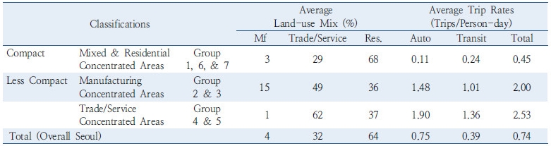
In order to examine these groups in terms of work-trip generation rates, the average rates of each group are calculated based on the KTDB 2010 and compared each other. The ANOVA (Analysis of Variance) technique is used to verify that the clusters are different from each other in the trip generation rates. As a result, 3 clusters are defined: mixed land-use area (group 1) and residentially concentrated area (group 6 and 7) as a compact area; manufacturing concentrated area (group 2 and 3); finally, trade & service concentrated area (group 4 and 5). The first cluster includes sub-districts with more balance land-use mix and high density of household. This cluster includes 358 sub-districts. The average proportions of manufacturing, trade & service, and residential sectors for this cluster are 3%, 29%, and 68% respectively. This is not so different from the overall pattern of the Seoul city: 4% in the manufacturing sector, 32% in trade & service sector, and 64% in the residential sector.

The second cluster represents manufacturing concentrated areas in which the proportion of manufacturing sectors is higher than other areas. In these areas, the manufacturing sector reaches over 15% while in other areas it generally does not exceed 4%. Sub-districts classified into this group have 49% of trade & service sectors and relatively low with 36% of the residential sector.

The last cluster represents trade & service concentrated areas. These areas have a relatively low proportion of manufacturing sector, which is only makeup 1%. Obviously, these areas have a high proportion of trade & service sector with 62%. However, the proportion of residential sector in these areas is relatively low with 37% similar to the areas in the second cluster.

Table 1. Land-use mix and work-trip generation rates by clusters

The areas of each cluster are statistically compared in terms of their trip generation rates by modes (auto and transit) in order to prove that the difference of urban compactness will result in different trip generation patterns. As stated before, besides identifying how many trips people in compact areas will make, this research also will determine whether people in compact areas will be more encouraged to use public transport. Table 2, 3, and 4 show that the areas of each cluster are significantly different from each other in terms of the trip generation rates by modes.

Table 2. Significance test of differences in work-trip generation rate

Table 3. Significance test of differences in work-trip generation rate by car

Table 4. Significance test of differences in work-trip generation rate by transit

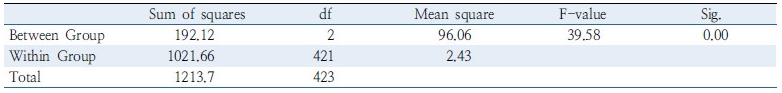
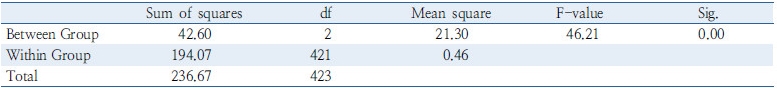
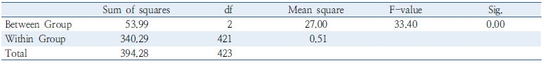
As can be seen in the ANOVA results in Tables 2, 3, and 4, it has statistical evidence in the level of significance 0.05 that the areas with different level of urban compactness will result with different level of trip generation rate. The post-hoc test has been actually conducted by using the Games-Howell test. This test is conducted to see further in which part the biggest differences happen. The output of Games-Howell tests is not included in this paper due to extensive results and they also show same results with F-test in ANOVA that the clustered groups are statistically different to each other.

Impacts of Compactness and Density on Work-Trip Generation

There are two comprehensions obtained from the above statistical analysis. First, the people in compact areas will generally make fewer trips compared to less compact areas. Second, the people in compact areas will use more public transport compared to private cars. Based on these, a multiple linear regression model is applied to explain the effects of urban compactness on travel pattern especially the trip generation of each area.

The dependent variable is trip generation rates by modes and the independent variables are the measurements of urban compactness for each of sub-districts. Also, some socio-economic data is used to effectively explain the trip generation patterns.

The categorized groups of urban compactness level of sub-district are classified by converting these groups into dummy variables. Hence, in the urban compactness level, there will 2 dummy variables as independent variables. The relatively more compact areas will be used as a comparison. Thus, dummy variable for the manufacture intensive area and trade & service intensive area will be shown in the multiple regression analysis models.

In addition to the variables representing the level of urban compactness, the Residential/Nonresidential Ratio (RNR) as the strengthening representative of density aspect, and some socio-economic variables are added. The RNR is calculated by using proxy variables, where the population is used instead of residential area, and the number of workers is used instead of the non-residential area. This variable is utilized to investigate whether the people who work in one area also live in the same area, or, at least, to identify the balance between the number of people who live and work in one area. Because this variable uses the population and worker ratios, it is arguably more effective in terms of their relationship to trip generations compared to conventional RNR which merely use the residential to the non-residential ratio which in high probability includes the non-essential type of land use as well. The RNR will be 1.0 for completely equal and otherwise less than 1.0. This proxy RNR will be calculated as follows (Modified from Jeong et al., 2013):

                (1)

Where R = number of population (person), NR = number of workers (person).

Also, some socio-economic variables, car-ownership, and the accessibility of subway are introduced in the initial steps of the stepwise multiple linear regression analysis.

The models show adequate R-square values. However, the variable for the availability of subway station is not significant statistically. The existence of this variable may give turbulence to other variables in the multiple linear regression models. Therefore, the analysis should be re-conducted by excluding this variable. Finally, the result can be seen in Table 5, 6, and 7 by modes.

Table 5. Impacts of urban compactness and residential density on work-trip generation: total

Table 6. Impacts of urban compactness and residential density on work-trip generation: by car

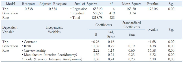
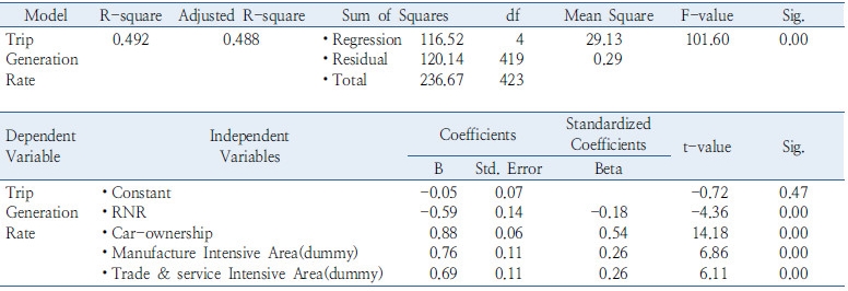
Table 7. Impacts of urban compactness and residential density on work-trip generation: by public transit

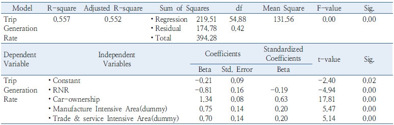The regression models explain trip generation 54% in total, 49% by car, and 56% by public transit. All of the models are statistically significant in 0.05. Car-ownership in the models shows positive. Increasing 1 car per household will result in 0.60 increase in trip generation rate overall, 0.54 by car, and 0.63 by transit.

The coefficients of RNR are all negative; -0.19, -0.18, and -0.19 in total and by modes respectively. This means that higher RNR will engender lower trip generation rate.

For the urban compactness, it can be seen that people in compact areas will do 0.20-0.26 fewer trips per person per day. However, the reduction of trip generation by car is higher compared to the reduction of trip generation by transit. People in compact areas will use fewer cars for work trips compared to manufacture intensive and trade & service intensive areas. In trips by transit, compact areas will have 0.20 fewer trip generation rates compared to manufacture intensive areas and trade & service intensive areas.

The overall results of regression analysis illustrate that increasing residential density (RNR) and urban compactness will reduce the demand for inter-zonal work trips. Additionally, the compact areas are also encouraging more people to use public transport instead of private cars.

Conclusions

The research results demonstrate that in the most comprehensive measurement of urban compactness, the mixed-use aspect can be utilized instead of merely focusing on density aspect. Also the better results can be achieved by classification of the data collection for urban compactness groups considers subdistrict's work-trip generation rate. Furthermore, the regression models show that the compact areas produce less inter-zonal trip generation rate by modes. However, the impacts of urban compactness on the work-trip generation shows that improving residential density (RNR) and urban compactness will be more effective to reduce the travel demand.

Throughout the study some limitations are also realized, which may be useful for future studies’ consideration. In this study, the urban compactness is measured by the number of employments and applied into the models by simple dummy variables. It may be useful to measure the urban compactness by other socio-economic data and to apply mode clear variables in the models. In addition, most of transportation demand models have not used the urban compactness variables as the explanatory variables. If we have more specified variables for the urban compactness, some new type of trip generation models can be developed by introducing the variables not only zonal socio-economic characteristics but zonal land-use patterns.