Journal of Korean Society of Transportation. April 2017.
https://doi.org/10.7470/jkst.2017.35.2.091

ABSTRACT


MAIN

  • 서론

  • 선행연구

  • 방법론 및 데이터

  •   1. GCAM의 개요 및 수송부문 모형

  •   2. 데이터 및 GCAM의 재구성

  • GCAM 재구성 결과

  • 결론

서론

2014년 전 세계 수송부문에서 사용한 에너지양은 2,672 MTOE이며, 그 중 1.3%인 37 MTOE의 양이 국내 수송부문에서 사용되었다. 특히 전 세계 수송부문 에너지사용의 92%가 석유 및 유류제품인데 반해, 국내 수송부문의 경우 95%가 석유 및 유류제품으로써, 전 세계 수송부문의 평균보다 석유 및 유류제품에 대한 의존이 다소 높다. (IEA, 2016), (KEEI, 2015) 국내 수송부문에서 배출한 탄소배출량은 87.5 MtC이며, 1990년부터 2013년까지 연평균 4%씩 꾸준한 증가추세를 보이고 있다(GIR, 2015). IPCC 5차보고서에 의하면, 적극적인 전 지구적 대응방안이 없는 경우, 전 세계 수송 부문에서의 탄소배출량이 7.0 GtC에서 2050년에는 12.0 GtC로 증가할 것으로 보고한 바 있다 (Sims et al., 2014). 이와 같이, 수송부문은 최종에너지 소비부문의 하나로, 화석에너지 사용 및 온실가스배출로 큰 부담을 주고 있다. 본 연구에서는 수송부문을 Global Change Assessment Model (GCAM) 이라는 통합모형을 활용하여 분석하고자 한다. 통합모형은 에너지시스템 전반의 구조를 유기적으로 구성함으로써, 타부문의 feedback효과 (예, 전기차 증가에 따른 전력생산 증가 및 전환부문의 에너지 믹스의 변화에 따른 온실가스배출계수 변화)까지도 함께 고려하여 시나리오분석을 한다는 특징이 있다. 통합모형에 대한 보다 자세한 내용은 선행연구로 대체하고자 한다*1). IPCC 등과 같은 국제기구에서 GCAM을 공인된 모형으로 활용하고 있다는 사실에 비추어 볼 때, GCAM이 통합모형으로써 충분한 활용가치가 있다고 판단된다. 하지만, GCAM에 내장되어 있는 국내 데이터가 현실과 동떨어진 부분이 있음을 확인할 수 있다. 따라서 본 연구는 GCAM의 국내 수송부문의 기본적인 입력 데이터가 현실과 부합하도록 모델링 함에 그 의의가 있다고 하겠다. 구체적으로는, 국가통계에 준거한 기준년도 서비스수요의 상세 설정, 이후 미래에 대한 기준 시나리오가 과거 추이를 제대로 반영하도록 하는 것이다.

선행연구

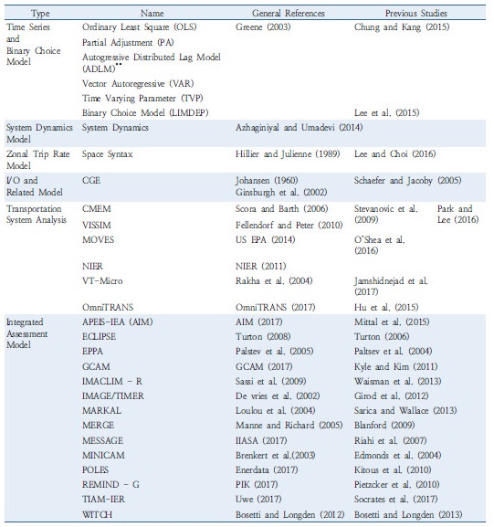
일반적으로 수송부문 모형이라 함은 다양한 모형을 포함한다. Table 1을 보면, 교통공학분야에서 널리 쓰이는 계량모형부터, 본 연구에서 활용한 통합모형까지 다양한 종류의 수송부문 모형을 소개하고 있다. Type별로 모형을 분류한 것은 De Jong et al.(2004)를 참고하였다. 이에 따르면, 수송부문 모형에 관해 기본적인 분류를 Trend and Time Series Model, System Dynamics Model, Zonal Trip Rate Model, I/O and related Model로 분류하고 있다. 본 연구에서는 선행연구 분류 체계에 Transportation System Analysis와 Integrated Assessment Model을 추가하여, 관련 문헌을 표로 요약 정리하였다. 본 연구에서 활용한 GCAM은 Integrated Assessment Model 중 하나로, Girod et al.(2013)을 참고하면, GCAM을 포함한 다양한 통합모형의 수송부문을 살펴 볼 수 있다. GCAM에 관한 보다 자세한 내용은 다음 장에서 언급하고자 한다.

Table 1. Models for transportation sector analysis

http://static.apub.kr/journalsite/sites/kst/2017-035-02/N0210350201/images/Table_KST_35_02_01_T1.jpg

Note: **ADLM is another presentation of ARDL in econometrics.

방법론 및 데이터

1. GCAM의 개요 및 수송부문 모형

GCAM은 Intergovernmental Panel on Climate Change(IPCC)의 제5차 평가보고서 작성의 기준시나리오가 되는 RCP4.5 작성에 활용된 바 있고**2), 상향식 모형으로 경제, 에너지시스템, 토지이용, 기후변화를 통합한 모형이다. 2010년을 기준년도로 하여 5년 단위로 2100년까지 시뮬레이션이 가능하며, 전 세계를 32개의 지역으로 구분하고 있고, 우리나라는 32개 지역들 중 하나의 단일지역으로 구분되어 있다. GCAM은 장기간의 기술평가를 목적으로 하고 있으며, 시나리오분석을 통한 정책적 함의를 도출하기 위해 활용되고 있다.***3) 본 연구에서 GCAM 통합모형을 사용하는 몇 가지 이유는 다음과 같다. 선행연구를 통해, 국내 에너지시스템을 구성하는 건물, 산업, 그리고 전환부문에 대한 상세 모형작업이 이루어져 있어****4), 수송부문에 대한 추가연구는 기존 연구와 통합한다는 측면에서 그 의의가 있다. 또한 여타 선형모형들과 달리, 경쟁 하의 기술 선택과정을 조건부 로짓함수로 모형화 함으로써, Keepin and Brian(1984)이 지적한 바와 같이, 선형모형에서 나타나는 극단적인 기술선택의 결과가 나타나지 않도록 하는 장점이 있다.

GCAM의 수송부문 모형은 여객과 화물부문으로 이루어져 있다*****5). 여객 서비스수요의 단위는 Passenger- Kilometer (PKM) 라고 하며, 화물 서비스수요의 단위는 Ton-Kilometer (TKM)로 표시한다. 그 이외, 운송수단이 주행한 총거리는 총주행거리, 혹은 Vehicle-Kilomter (VKM) 이라고 표시한다. 여객부문과 화물부문의 서비스수요는 모형 내에서 각각 다음과 같이 계산된다.

여객부문의 서비스수요: http://static.apub.kr/journalsite/sites/kst/2017-035-02/N0210350201/images/PIC80D2.gif

(1)

화물부문의 서비스수요: http://static.apub.kr/journalsite/sites/kst/2017-035-02/N0210350201/images/PIC8160.gif

(2)

여기서, http://static.apub.kr/journalsite/sites/kst/2017-035-02/N0210350201/images/PIC8180.gif는 해당부문의 서비스수요, http://static.apub.kr/journalsite/sites/kst/2017-035-02/N0210350201/images/PIC81B0.gif는 캘리브레이션 파라미터, http://static.apub.kr/journalsite/sites/kst/2017-035-02/N0210350201/images/PIC81E0.gif는 1인당 소득, http://static.apub.kr/journalsite/sites/kst/2017-035-02/N0210350201/images/PIC823F.gif는 수송서비스가격, http://static.apub.kr/journalsite/sites/kst/2017-035-02/N0210350201/images/PIC825F.gif은 인구 수, http://static.apub.kr/journalsite/sites/kst/2017-035-02/N0210350201/images/PIC8270.gif는 총소득을 나타낸다. http://static.apub.kr/journalsite/sites/kst/2017-035-02/N0210350201/images/PIC8280.gif는 년도, http://static.apub.kr/journalsite/sites/kst/2017-035-02/N0210350201/images/PIC8291.gif는 소득탄력성, http://static.apub.kr/journalsite/sites/kst/2017-035-02/N0210350201/images/PIC82A2.gif는 가격탄력성을 나타낸다. 소득 및 인구에 대한 가정은 SSP2 (Shared Socioeconomic Pathways)를 가정하였다*6). Equation(1)과 Equation(2) 에서 가격변수 만이 모형에서 내생적으로 결정되는 변수이다. 특히 가격변수는 기술을 평가함에 있어 가장 중요한 변수로 작용하므로, 자세히 살펴 볼 필요가 있다. 수송서비스 가격은 다음과 같은 방식으로 계산 된다.

http://static.apub.kr/journalsite/sites/kst/2017-035-02/N0210350201/images/PIC82C2.gif

http://static.apub.kr/journalsite/sites/kst/2017-035-02/N0210350201/images/PIC82D2.gif

http://static.apub.kr/journalsite/sites/kst/2017-035-02/N0210350201/images/PIC82F3.gif

http://static.apub.kr/journalsite/sites/kst/2017-035-02/N0210350201/images/PIC8303.gif

(3)

여기서, 각 변수들은 수송모드의 종류(http://static.apub.kr/journalsite/sites/kst/2017-035-02/N0210350201/images/PIC8324.gif), 크기(http://static.apub.kr/journalsite/sites/kst/2017-035-02/N0210350201/images/PIC8334.gif), 기술(http://static.apub.kr/journalsite/sites/kst/2017-035-02/N0210350201/images/PIC8345.gif), 연료가격(http://static.apub.kr/journalsite/sites/kst/2017-035-02/N0210350201/images/PIC8355.gif, $/MJ), 비연료가격(http://static.apub.kr/journalsite/sites/kst/2017-035-02/N0210350201/images/PIC8376.gif, $/VKT), energy intensity(http://static.apub.kr/journalsite/sites/kst/2017-035-02/N0210350201/images/PIC8386.gif, MJ/VKT), load factor(http://static.apub.kr/journalsite/sites/kst/2017-035-02/N0210350201/images/PIC8397.gif, PKM/VKM**7)), 시간당임금(http://static.apub.kr/journalsite/sites/kst/2017-035-02/N0210350201/images/PIC83A8.gif, $/hour), 속도(http://static.apub.kr/journalsite/sites/kst/2017-035-02/N0210350201/images/PIC83B8.gif, KM/hour), 기술점유율(http://static.apub.kr/journalsite/sites/kst/2017-035-02/N0210350201/images/PIC83C9.gif)을 나타낸다. Equation(3)에서 수송모드의 기술점유율인 http://static.apub.kr/journalsite/sites/kst/2017-035-02/N0210350201/images/PIC83D9.gif가 GCAM에서 모사하는 사실상 기술경쟁의 결과 값으로, 매우 중요한 변수이다. 이는 다음과 같이 로짓모형을 통해 계산 된다.***8)

http://static.apub.kr/journalsite/sites/kst/2017-035-02/N0210350201/images/PIC83FA.gif

(4)

여기서, 각 변수들은 수송모드의 기술점유율(http://static.apub.kr/journalsite/sites/kst/2017-035-02/N0210350201/images/PIC840A.gif), share weight(http://static.apub.kr/journalsite/sites/kst/2017-035-02/N0210350201/images/PIC841B.gif), 로짓지수(http://static.apub.kr/journalsite/sites/kst/2017-035-02/N0210350201/images/PIC842C.gif)를 나타낸다. 앞서 설명한 GCAM 수송부문 모형은 서비스수요를 시뮬레이션 하는 과정이다. Equation(1), Equation(2) 에서 서비스수요와 에너지소비의 연계 과정은 서비스수요 항등식을 통해 이루어지며, Equation(5)와 같다.****9)

http://static.apub.kr/journalsite/sites/kst/2017-035-02/N0210350201/images/PIC849A.gif

(5)

여객 수송서비스의 경우, 상기 각 변수들은 에너지사용량(http://static.apub.kr/journalsite/sites/kst/2017-035-02/N0210350201/images/PIC84AB.gif, calorific value), 연비(http://static.apub.kr/journalsite/sites/kst/2017-035-02/N0210350201/images/PIC84BB.gif, VKM/calorific value), load factor(http://static.apub.kr/journalsite/sites/kst/2017-035-02/N0210350201/images/PIC84CC.gif, PKM/VKM)를 나타낸다. Equation(5)는 Kaya 항등식을 수송부문에 적용했음을 알 수 있다. Kaya(1990)에 제시된 Kaya 항등식은 하나의 변수를 여러 가지 요인으로 분해하여 설명할 수 있다는 장점을 가지고 있다. 하지만, rebound effect의 문제가 발생할 수 있음도 지적되고 있다.*****10) 대표적인 예로서, 특정 수송모드의 에너지효율향상은 직접적인 효과로 해당 수송모드의 에너지사용량을 감소시키지만, 간접적으로는 에너지효율의 향상으로 인한 가격하락은 소비자로 하여금 그 수송모드의 사용을 증가시킬 여지가 있다. 본 연구에서 에너지사용량(http://static.apub.kr/journalsite/sites/kst/2017-035-02/N0210350201/images/PIC84DC.gif), 총주행거리(http://static.apub.kr/journalsite/sites/kst/2017-035-02/N0210350201/images/PIC84ED.gif), 서비스수요(http://static.apub.kr/journalsite/sites/kst/2017-035-02/N0210350201/images/PIC84FE.gif) 정보는 국가통계를 활용하였고, 수송모드의 세분화 과정의 loadfactor(http://static.apub.kr/journalsite/sites/kst/2017-035-02/N0210350201/images/PIC850E.gif)는 상기의 Equation(5)를 만족시키는 값들로 설정하였다. 관련 상세 내용은 다음 장에서 설명한다.

2. 데이터 및 GCAM의 재구성

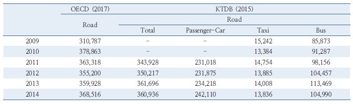
Table 2에 제시된 국내 수송부문 서비스수요 데이터는 KTDB(2015)에서도 확인이 가능하며, OECD(2017)에서도 도로와 철도 부문에 한해 확인이 가능하다. 두 통계간의 차이가 발생하는 것을 볼 수 있는데, 이는 실제 교통조사 시 차종의 구분 문제로 인한 것임을 확인하였다.*11) KTDB에서 보고 되지 않는 2010년의 Passenger-Car의 서비스수요의 경우, 2011년 Passenger-Car의 서비스수요와 같다고 가정하였다. Table 3은 본 연구에서 Equation(5)를 활용하여 얻은 서비스수요, 에너지사용량, 총주행거리, loadfactor의 값을 실제 통계수치와 비교하고 있다.
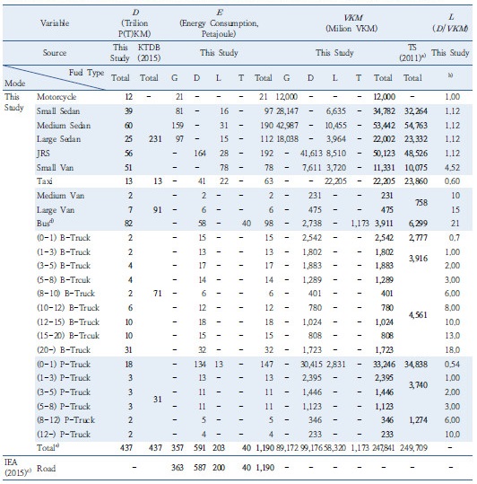
Table 2. Comparison of service demand statistics in passenger road sector (unit: milion PKM)

http://static.apub.kr/journalsite/sites/kst/2017-035-02/N0210350201/images/Table_KST_35_02_01_T2.jpg

Table 3. Data comparison between this study and statistics; demand, energy consumption, vehicle-kilometer, loadfactor

http://static.apub.kr/journalsite/sites/kst/2017-035-02/N0210350201/images/Table_KST_35_02_01_T3.jpg

※ Rather than road sector, the others are also available upon request.

※ Acronym- G:Gasoline, D:Diesel, L:LPG, T:Town gas

a): TS(2011), Chap.4.1. b): Regardless of the each mode’s fuel type, loadfactor is assumed to be the same. c):The transportation sector is divided only upto the bigger categories of roads, railways, ships, airplanes, international ships, and airplanes in IEA energy balance table. Energy Census Report (KEEI, 2012) is utilized for further detailed classification. (d): Even if the VKM of bus fueled by gas is about 60% different between ‘This Study’ and ‘TS(2011)’, fuel efficiency of the mode is assumed 1.30(KM/Nm3) referring to Kim et al.(2013), refer the Kim et al.(2013) (e): The total value is without counting of Motorcycle case to compare with KTDB(2015)

서비스수요(http://static.apub.kr/journalsite/sites/kst/2017-035-02/N0210350201/images/PIC852F.gif)와 총주행거리(http://static.apub.kr/journalsite/sites/kst/2017-035-02/N0210350201/images/PIC853F.gif) 정보는 국가교통DB센터에서 매년 발간하는 국가교통통계 (KTDB, 2015)를 활용하였다. 에너지사용량(http://static.apub.kr/journalsite/sites/kst/2017-035-02/N0210350201/images/PIC8550.gif)의 경우, GCAM에서도 IEA (International Energy Agency)의 에너지 밸런스 표를 기본으로 하는 바, 본 연구에서도 IEA의 에너지 밸런스 표를 활용한다. 다만 수송부문의 세분화를 위하여, 에너지경제연구원에서 4년마다 발행하는 에너지총조사 보고서를 함께 참조하였다.

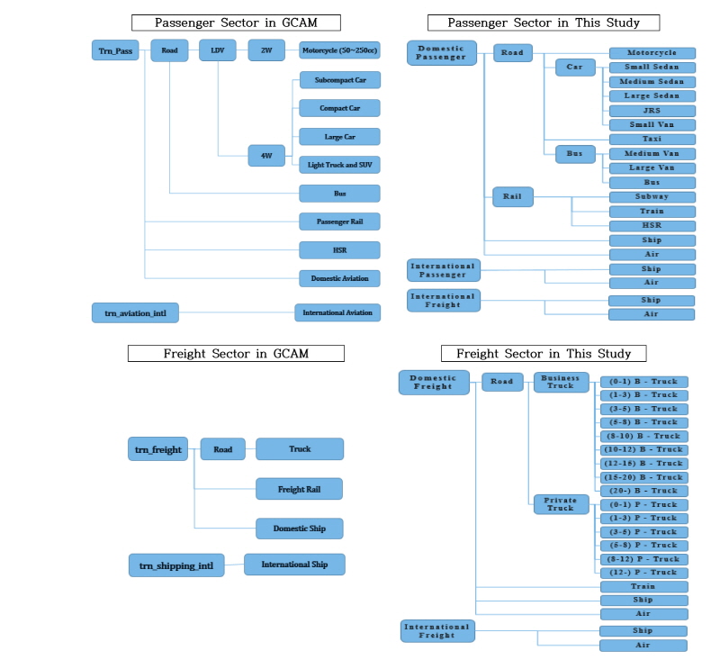
Figure 1은 기존 GCAM과 본 연구에서 사용한 수송부문 구조를 비교하고 있다. 여객부문의 경우 택시, 소·중·대형 승합차(van), 지하철, 국내선박, 국제선박이 추가 되었다. 승합차의 경우 국내에서는 소형 승합차(15인승 이하)는 승용차로 분류되며, 중·대형 승합차는 버스로 분류 된다**12). 화물부문의 경우 트럭이 영업용과 자가용으로 분류되었고, 나아가 적재별로 세분화되었다. 화물부문 또한 GCAM에서는 화물항공을 모델링하지 않았지만, 본 연구에서는 추가적으로 국내 화물항공, 국제 화물항공 부문을 모델링 하였다.

http://static.apub.kr/journalsite/sites/kst/2017-035-02/N0210350201/images/Figure_KST_35_02_01_F1.jpg
Figure 1.

Comparison of transportation structure. ※JRS: Jeep · Recreation vehicle · SUV, B-Truck: Business Truck, P-Truck: Private Truck

GCAM 재구성 결과

Figure 2는 도로와 철도부문의 서비스수요 과거추이와 시뮬레이션결과를 국제비교를 통해 보여주고 있다. http://static.apub.kr/journalsite/sites/kst/2017-035-02/N0210350201/images/PIC85ED.PNG 표식은 국내의 각 수송부문 과거 추이이며, 붉은색 중 http://static.apub.kr/journalsite/sites/kst/2017-035-02/N0210350201/images/PIC85FE.PNG 표식은 원래 GCAM의 시뮬레이션 결과인 반면, http://static.apub.kr/journalsite/sites/kst/2017-035-02/N0210350201/images/PIC861E.PNG표식은 본 연구의 결과이다. 우상단의 여객철도 부문을 제외하고, 모든 부문에서 기준년도 서비스수요와 GCAM의 시뮬레이션 서비스수요와 큰 차이가 있음을 확인 할 수 있다. 또 화물도로 부문을 제외하고, 모든 부문에서 GCAM 시뮬레이션 결과는 과거 서비스수요의 추이와 많은 차이를 보이고 있음을 확인할 수 있다.

http://static.apub.kr/journalsite/sites/kst/2017-035-02/N0210350201/images/Figure_KST_35_02_01_F2.jpg
Figure 2.

GDP per capita vs demand per capita. domestic road and rail sector

 상기와 같은 방법으로 여객, 화물 수송서비스의 장기 추이를 비교한 연구로는 Schipper et al.(1997)를 포함, 다양한 연구들***13)이 있다. 특히, Girod et al.(2013)에서는 비교뿐만 아니라 이를 통해 미래 추이를 결정하고, 시뮬레이션을 진행한 결과를 보여주고 있다.

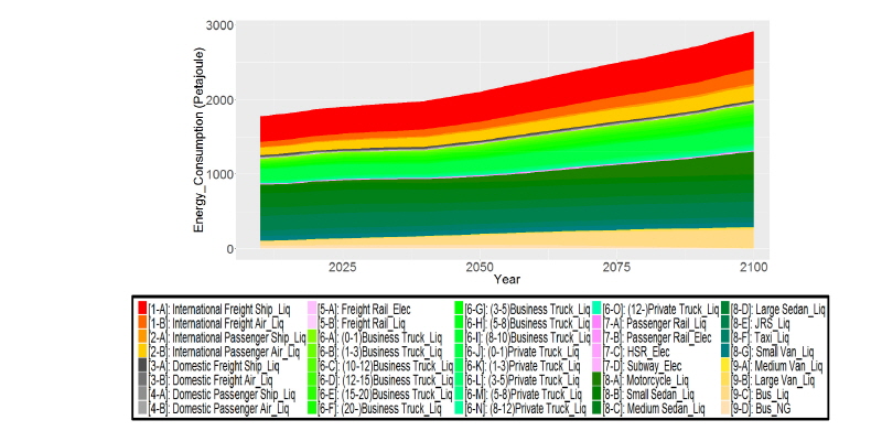
Figure 3은 에너지수요에 대한 시뮬레이션 결과이다. 기준년도의 에너지소비가 1,777PJ인데 반해, 2030년 1,930PJ, 2050년 2,102PJ, 그리고 2100년에 2,914으로 기준년도 대비 각각 8.5%, 18%, 그리고 64% 증가하는 것으로 나타났다.

http://static.apub.kr/journalsite/sites/kst/2017-035-02/N0210350201/images/Figure_KST_35_02_01_F3.jpg
Figure 3.

Energy consumption by technologies in this study

결론

본 연구에서는 통합모형인 GCAM을 활용한 국내 수송부문 모델링에 관한 문제를 논의하였다. 본 연구에 활용된 GCAM은 소스 데이터 및 코드가 공개되어 있으나, 수송부문의 상세 기준년도 정보를 제대로 반영하고 있지 못할 뿐만 아니라, 국내 수송서비스수요의 국가통계상 과거추이도 제대로 반영하고 있지 못하다는 문제가 있다. 따라서 이를 국내 수송부문 분석에 바로 적용하여 활용하기에는 여러 문제가 있다는 점이 본 연구의 동기가 되었다. 이에 본 연구에서는 수송부문 서비스수요 항등식을 통하여, 기준년도의 서비스수요를 국가교통통계와 일치하도록 모델링하였다. 본 연구는 전체 에너지시스템의 한 축을 구성하고 있는 국내 수송부문을 세분화하는 모델링 자체에 그 주안점이 있다. 따라서 이를 근거로 향후 특정정책에 대한 평가 등 추가적인 연구를 진행할 수 있는 기틀을 제공한다는데 그 의의가 있다고 하겠다. 본 연구의 결과는 기본적으로는 BAU (Business as Usual) 기준안에서 예상되는 여객 및 화물수송서비스의 세부수요를 중장기적 측면에서 설명해 낼 수 있고, 관련 에너지원별 수요 및 온실가스정보도 함께 산정할 수 있으며, 외부적인 정책변화에 따른 효과 평가에 활용할 수 있다. 그 한 가지 사례로, 정부에서는 2016년 12월에 발표한 ‘제1차 기후변화대응 기본계획’을 통해, 수송부문에 주어진 과제가 승용차 및 중대형차 평균연비 개선, 친환경차 보급, 대중교통 운영확대 등으로 제시한 바 있으며, 이에 대한 정량적 평가에 이용할 수 있다. 즉, 본 연구의 결과를 기준안으로 삼고, 정부정책으로 제시된 개별정책을 각각의 대안 시나리오로 하여, 정책 집행에 따른 각 에너지시스템 구성요소, 에너지 및 온실가스배출 측면의 변화에 대한 분석이 가능하게 된다.

*) Moss et al.(2010), van Vuuren et al.(2011a), Edmonds and Reiley(1985), Edmonds et al.(1997), Kim et al.(2006) 참조.

**) van Vuuren et al.(2011b) 참조

***) 상세한 설명은 GCAM(2017) 참조

****) Baek et al.(2015, 2016) 참조

*****) Mishra et al.(2013) 참조

*) GCAM(2017), Ebi et al.(2014) 참조

**) 화물 수송서비스를 나타내는 경우는 TKM/VKM 임.

***) GCAM에서 해당 기술선택 관련 이론적 설명은 Clark et al.(1993)을 참조,

****) 편의상 위, 아래첨자 제외함.

*****) Wang et al.(2012), Sorrell et al.(2009) 참조

*1) 국가교통DB센터 고두환 연구원.

**) 국토부의 12종 교통량조사 차종분류가이드: http://www.molit.go.kr/USR/policyTarget/m_24066/dtl.jsp?idx=161

***)SCHIPPER et al.(1997)은 Figure 2에서 USA, Japan, Denmark, EU-4, NO-4를 비교하였고, Kamakate' et al.(2009)은 Figure 1, 3에서 USA, UK 그리고 Japan 등 5개국, Eom et al.(2010)은 Figure 3-6에서 한국을 포함한 8 개 국가, Millard-Ball et al.(2011)은 Figure 7에서 USA, Cananda 등 8개 국가, Kyle et al.(2011)은 Figure 1에서 한국을 포함하여 14개 국가, 그리고 Eom et al.(2012)은 Figure 2,3에서 11개 IEA국가들에 대한 장기 추이를 비교함.

Acknowledgements

Authors’ thanks go to Dr.Oh, Dr.Yurnaidi, Mr.Baek and Ms.Roh for carrying out the GCAM modeling work used in this study. Authors also would like to thank Doo Hwan Ko, KOTI researcher, for his kind help and three anonymous reviewers for clarifying important issues through the peer review process.

References

1
AIM, Asia-Pacific Integrated Model, http://www-iam.nies.go.jp/aim/ [Accessed: Feb.09,2017]
2
Azhaginiyal A., Umadevi G. (2014), System Dynamics Simulation Modeling of Transport, Energy and Emissions Interactions, Civil Engineering and Architecture, 2(4), 149-165.
3
Baek M., Oh J., Kim S. (2015), Analyzing the Long-Term Impact of Energy Efficiency Improvement Programs on Large Commercial Buildings Using GCAM-EML, Korean Energy Economic Review, 53(1), 33-67.
4
Baek M., Rho M., Yurnaidi Z., Kim S. (2016), Abatement Potentials of Power Generation Technologies for the Achievement of National INDC, Environmental and Resource Economic Review, 25(4), 565-590.
5
Blanford G. J., Richels R. G., Rutherford T. F. (2009), Feasible Climate Targets: The Roles of Economic Growth, Coalition Development and Expectations, Energy Economics, 31, S82-S93.
6
Bosetti V., Catenacci M., Fiorese G., Verdolini E. (2012), The Future Prospect of PV and CSP Solar Technologies: An Expert Clicitation Survey, Energy Policy, 49, 308-317.
7
Bosetti V., Longden T. (2013), Light Duty Vehicle Transportation and Global Climate Policy: The Importance of Electric Drive Vehicles, Energy Policy, 58, 209-219.
8
Brenkert A., Smith S., Kim S., Pitcher H. (2003), Model Documentation for the MiniCAM, Pacific Northwest National Laboratory Richland, WA.
9
Chung S.H., Kang K.W. (2015), A Comparative Study on the Forecasting Accuracy of Econometric Models: Domestic Total Freight Volume in South Korea, J. Korean Soc. Transp., 33(1), Korean Society of Transportation, 61-69.
10
Clarke J.F., Edmonds J.A. (1993), Modelling Energy Technologies in a Competitive Market, Energy Economics, 15(2), 123-129.
11
De Jong G., Gunn H., Walker W. (2004), National and International Freight Transport Models: An Overview and Ideas for Future Development, Transport Reviews, 24(1), 103-124.
12
De Vries, B., van Vuuren, D., Den Elzen, M., Janssen, M. (2002), Targets IMage Energy Regional (TIMER) Model, Technical Documentation.
13
Ebi K. L., Hallegatte S., Kram T., Arnell N. W., Carter T. R., Edmonds J., Winkler H. (2014), A New Scenario Framework for Climate Change Research: Background, Process, and Future Directions, Climatic Change, 122(3), 363-372.
14
Edmonds J., Clarke J., Dooley J., Kim S. H., Smith S. J. (2004), Stabilization of CO 2 in a B2 World: Insights on the Roles of Carbon Capture and Disposal, Hydrogen, and Transportation Technologies, Energy Economics, 26(4), 517-537.
15
Edmonds J., Reilly J. (1985), Global Energy: Assessing the Future (Oxford University Press, New York), 317.
16
Edmonds J., Wise M., Pitcher H., Richels R., Wigley T., MacCracken C. (1997), An Integrated Assessment of Climate Change and the Accelerated Introduction of Advanced Energy Technologies, Mitigation and Adaptation Strategies for Global Change, 1, 311-339.
17
Enerdata, POLES, https://www.enerdata.net/solutions/poles-model.html [Accessed: Feb.09,2017]
18
Eom J., Schipper L. (2010), Trends in Passenger Transport Energy Use in South Korea, Energy Policy, 38(7), 3598-3607.
19
Eom J., Schipper L., Thompson L. (2012), We keep on truckin': Trends in Freight Energy Use and Carbon Emissions in 11 IEA Countries, Energy Policy, 45, 327-341.
20
Fellendorf M., Vortisch P. (2010), Microscopic Traffic Flow Simulator VISSIM, Fundamentals of Traffic Simulation, Springer New York, 63-93.
21
GCAM, Global Change Assessment Model, http://www.globalchange.umd.edu/archived-models/gcam/, http://jgcri. github.io/gcam-doc/index.html [Accessed: Feb.09,2017]
22
Ginsburgh V., Keyzer M. (2002), The Structure of Applied General Equilibrium Models, MIT Press.
23
GIR (2015), National Greenhouse Gas Inventory Report of Korea, Greenhouse Gas Inventory & Research Center of Korea
24
Girod B., van Vuuren D. P., Deetman S. (2012), Global Travel Within the 2 C Climate Target, Energy Policy, 45, 152-166.
25
Girod B., van Vuuren D. P., Grahn M., Kitous A., Kim S. H., Kyle P. (2013), Climate Impact of Transportation a model Comparison, Climatic Change, 118(3-4), 595-608.
26
Greene H. W. (2003), Econometric Analysis, New Jersey: Prentice Hall.
27
Hillier B., Hanson J. (1989), The Social Logic of Space, Cambridge University Press.
28
Hu H., Yang C., Yoon C., Kim I., Sung J. (2015), Developing a Method for Estimating Urban Environmental Impact Using an Integrated Land Use-Transport Model, J. Korean Soc. Transp., 33(3), Korean Society of Transportation, 294-303.
29
IEA (2015), World energy balances, http://dx.doi.org/10.1787/data-00512-en, [Accessed: Feb.09,2017]
30
IEA (2016), Key world energy statistics, International Energy Agency
31
IIASA, MESSAGE, http://www.iiasa.ac.at/web/home/research/modelsData/MESSAGE/MESSAGE.en.html [Accessed: Feb.09,2017]
32
Jamshidnejad A., Papamichail I., Papageorgiou M., De Schutter B. (2017), A Mesoscopic Integrated Urban Traffic Flow-emission Model, Transportation Research Part C: Emerging Technologies, 75, 45-83.
33
Johansen L. (1960), A Multisectoral Study of Economic Growth (1ed.), Amsterdam: North-Holland.
34
Kamakaté F., Schipper L. (2009), Trends in Truck Freight Energy Use and Carbon Emissions in Selected OECD Countries From 1973 to 2005, Energy Policy, 37(10), 3743-3751.
35
Kaya H. K. (1990), Soil Ecology, Entomopathogenic Nematodes in Biological Control, 93-115.
36
KEEI (2012), 2011 Energy Consumption Survey (2011년도 에너지총조사 보고서), Korea Energy Economics Institute.
37
KEEI (2015), Yearbook of Energy Statistics, Korea Energy Economics Institute.
38
Keepin B., Wynne B. (1984) Technical Analysis of IIASA Energy Scenarios, Nature 312, 691-695.
39
Kim H. J., Sung B. J. (2013), Development of CNG Hybrid City Bus, Journal of the Korean Society of Automotive Engineers 35(2), 18-23.
40
Kim S.H., Edmonds J., Lurz J., Smith S. J., Wise M. (2006), The Objects Framework for Integrated Assessment: Hybrid Modeling of Transportation, Energy Journal (Special Issue #2), 51-80.
41
Kitous A., Criqui P., Bellevrat E., Chateau B. (2010), Transformation Patterns of the Worldwide Energy System-Scenarios for the Century With the POLES Model, The Energy Journal, 49-82.
42
KTDB (2015), 2014 Korea Transportation Statistics (2014 국가교통통계), Korea Transport Data Base.
43
Kyle P., Kim S. H. (2011), Long-Term Implications of Alternative Light-Duty Vehicle Technologies for Global Greenhouse Emissions and Primary Energy Demands, Energy Policy 39, 3012-3024.
44
Kypreos S., Glynn J., Panos E., Giannidakis G., O Gallachoir B., Energy, Climate Change and Local Atmospheric Pollution Scenarios Evaluated with the TIAM-MACRO Model, https://iea-etsap.org/projects/TIAM_Global_ CC&LAPScenarios-8616.pdf [Accessed: Feb.09,2017]
45
Lee K. S., Chung S. B., Eom J. K., Namkung B. K., Kim S. W. (2015), Development of Mode Choice Model for the Implementation of Next-generation High Speed Train(HEMU-430X), J. Korean Soc. Transp., 33(5), Korean Society of Transportation, 461-469.
46
Lee K.J., Choi K. (2016), Mobile Source Emissions Estimates for Intra-Zonal Travel Using Space Syntax Analysis, J. Korean Soc. Transp., 34(2), Korean Society of Transportation, 107-122.
47
Loulou R., Goldstein G., Noble K. (2004), Documentation for the MARKAL Family of Models, Energy Technology Systems Analysis Programme, 65-73.
48
Manne A. S., Richels R. G. (2005), MERGE: An Integrated Assessment Model for Global Climate Change, Energy and Environment, Springer US, 175-189.
49
Millard-Ball A., Schipper L. (2011), Are We Reaching Peak Travel? Trends in Passenger Transport in Eight Industrialized Countries, Transport Reviews, 31(3), 357-378.
50
Mishra G.S., Kyle P., Teter J., Morrison G.M., Yeh S., Kim S. (2013), Transportation Module of Global Change Assessment Model (GCAM): Model Documentation Version 1.0, Institute of Transportation Studies, University of California at Davis and Pacific Northwest National Laboratory, Report UCD-ITS-RR-13-05.
51
Mittal S., Hanaoka T., Shukla P. R., Masui T. (2015), Air Pollution Co-benefits of Low Carbon Policies in Road Transport: a Sub-national Assessment for India, Environmental Research Letters, 10(8), 085006.
52
Moss R. H., Edmonds J., Hibbard K. A., Manning M. R., Rose S. K., Van Vuuren D. P., Meehl G. A. (2010), The Next Generation of Scenarios for Climate Change Research and Assessment, Nature, 463(7282), 747-756.
53
NIER (2011), http://webbook.me.go.kr/DLi-File/NIER/06/013/5511438.pdf [Accessed: Feb.09,2017]
54
O’Shea W., Mueller S., Caldwell I., Lin J. (2016), Evaluation of the USEPA MOVES Model Sensitivity to Ethanol Fuel Blends: A Case Study in Cook County, Illinois, In Transportation Research Board 95th Annual Meeting (No.16-4146).
55
OECD, Transport data, https://data.oecd.org/transport/passenger-transport.htm [Accessed: Feb.09,2017]
56
OmniTRANS, OmniTRANS 8.0, http://www.dat.nl/en/products/omnitrans/80/ [Accessed: Feb.09,2017]
57
Paltsev S., Reilly J. M., Jacoby H. D., Eckaus R. S., McFarland J. R., Sarofim M. C., Babiker M. H. (2005), The MIT Emissions Prediction and Policy Analysis (EPPA) Model: Version 4, MIT Joint Program on the Science and Policy of Global Change.
58
Paltsev S., Viguier L., Babiker M., Reilly J., Tay K. H. (2004), Disaggregating Household Transport in the MIT-EPPA Model, MIT Joint Program on the Science and Policy of Global Change, Technical Note, 5.
59
Park S., Lee J. (2016), Evaluation of Fuel Consumption Models for Eco-friendly Traffic Operations Strategies, J. Korean Soc. Transp., 34(3), Korean Society of Transportation, 234-247.
60
Pietzcker R., Moll R., Bauer N., Luderer G. (2010, August), Vehicle Technologies and Shifts in Modal Split as Mitigation Options Towards a 2 C Climate Target, In Contribution to the 2010 ISEE Conference, Advancing Sustainability in a Time of Crisis, 22-25.
61
PIK, REMIND, https://www.pik-potsdam.de/research/sustainable-solutions/models/remind [Accessed: Feb.09,2017]
62
Rakha H., Ahn K., Trani A. (2004), Development of VT-Micro Model for Estimating Hot Stabilized Light Duty Vehicle and Truck Emissions, Transportation Research Part D: Transport and Environment, 9(1), 49-74.
63
Riahi K., Grübler A., Nakicenovic N. (2007), Scenarios of Long-term Socio-economic and Environmental Development Under Climate Stabilization, Technological Forecasting and Social Change, 74(7), 887-935.
64
Sarica K., Tyner W. E. (2013), Analysis of US Renewable Fuels Policies Using a Modified MARKAL Model, Renewable Energy 50, 701-709.
65
Sassi O., Crassous R., Hourcade J. C., Gitz V., Waisman H., Guivarch C. (2009), IMACLIM-R: A Modelling Framework to Simulate Sustainable Development Pathways, International Journal of Global Environmental Issues, 10(1-2), 5-24.
66
Schaefer A., Jacoby H. D. (2005), Technology Detail in a Multisector CGE Model: Transport Under Climate Policy, Energy Economics, 27(1), 1-24.
67
Schipper L., Scholl L., Price L. (1997), Energy Use and Carbon Emissions From Freight in 10 Industrialized Countries: An Analysis of Trends From 1973 to 1992, Transportation Research Part D, Transport and Environment, 2(1), 57-76.
68
Scora G., Barth M. (2006), Comprehensive Modal Emissions Model(CMEM), Version 3.01 User Guide, Centre for Environmental Research and Technology, University of California, Riverside.
69
Sims R., Schaeffer R., Creutzig F., Cruz-Núñez X., D’Agosto M., Dimitriu D., Figueroa Meza M. J., Fulton L., Kobayashi S., Lah O., McKinnon A., Newman P., Ouyang M., Schauer J. J., Sperling D., Tiwari G. (2014), Transport. In: Climate Change 2014: Mitigation of Climate Change, Contribution of Working Group III to the Fifth Assessment Report of the Intergovernmental Panel on Climate Change [Edenhofer O., Pichs-Madruga R., Sokona Y., Farahani E., Kadner S., Seyboth K., Adler A., Baum I., Brunner S., Eickemeier P., Kriemann B., Savolainen J., Schlömer S., von Stechow C., Zwickel T., Minx J.C. (eds.)], Cambridge University Press, Cambridge, United Kingdom and New York, NY, USA.
70
Sorrell S., Dimitropoulos J., Sommerville M. (2009), Empirical Estimates of the Direct Rebound Effect: A Review, Energy policy, 37(4), 1356-1371.
71
Stevanovic A., Stevanovic J., Zhang K., Batterman S. (2009), Optimizing Traffic Control to Reduce Fuel Consumption and Vehicular Emissions: Integrated Approach With VISSIM, CMEM, and VISGAOST, Transportation Research Record, Journal of the Transportation Research Board, (2128), 105-113.
72
TS (Korea Transportation Safety Authority) (2011), 2010 Automobile Mileage Analysis (2010년도 자동차 주행거리 실태분석 연구), http://www.ts2020.kr/tsk/rck/InqDetPTRTrafficSafety.do?bbsSn=4280&bbsCd=110&ctgCd=-1.
73
Turton H. (2006), Sustainable Global Automobile Transport in the 21st Century: An Integrated Scenario Analysis, Technological Forecasting and Social Change, 73(6), 607-629.
74
Turton H. (2008), ECLIPSE: An Integrated Energy-economy Model for Climate Policy and Scenario Analysis, Energy, 33(12), 1754-1769.
75
US EPA. (2014), Motor Vehicle Emission Simulator (MOVES) User Guide for MOVES2014.
76
Uwe Remme, Markus Blesl, Anjana Das, Ulrich Fahl, Overview of the Application of TIMES at IER, http://iea-etsap.org/workshop/worksh7-7/ier-overviewapplictimes.pdf [Accessed: Feb.09,2017]
77
van Vuuren D. P., Edmonds J. A., Kainuma M., Riahi K., Thomson A., Hibbard K., George C. H., Kram T., Krey V., Lamarque J.-F., Masui T., Meinshause M., Nakicenovic N., Smith S. J., Rose S. K. (2011b), Special Issue, The Representative Concentration Pathways: An Overview, Climatic Change, 109(1-2).
78
van Vuuren D. P., Lowe J., Stehfest E., Gohar L., Hof A. F., Hope C., Plattner G. K. (2011a), How Well Do Integrated Assessment Models Simulate Climate Change?, Climatic Change, 104(2), 255-285.
79
Waisman H. D., Guivarch C., Lecocq F. (2013), The Transportation Sector and Low-carbon Growth Pathways: Modelling Urban, Infrastructure, and Spatial Determinants of Mobility, Climate Policy, 13, 106-129.
80
Wang H., Zhou P., Zhou D. Q. (2012), An Empirical Study of Direct Rebound Effect for Passenger Transport in Urban China, Energy Economics, 34(2), 452-460.
페이지 상단으로 이동하기