Introduction

Unexpected incidents or accidents occur irregularly. They may cause or arise from traffic accidents, broken vehicles, wastes on a road, temporary road maintenance or repair and other non-routine events. An unexpected incident, meanwhile, will break down a steady traffic flow, causing a temporary decrease in the effective capacity of the road. For example, Sinha et al.(2007) simulated that an unexpected incident on blocking an one of three lanes may reduce the road capacity by about 50%, and upon the similar occasion Knoop et al.(2008) found empirical reduction of the road capacity up to about 65%. Therefore, when an incident occurs, an exact detection of the incident is considered to be the basic and essential subject for rapid reactions and dealings thereof.

In order to detect such unexpected incidents, this study aims to describe the 3-detector simplification model, proven by Daganzo(1997), in a statistical model and to verify the statistical appropriacy thereof. The Newell's 3-detector Simplification Method(NTSM) justified by Daganzo(1997) is applied in this study for detecting unexpected incidents. The applied method of detecting incidents in this study has variables, such as, the cumulative traffic flow with relatively less errors than the other attributes of traffic flows, and it enables to get prepared for detector data errors, which occur easily in high-density and highly occupied traffic flows, and provides the mathematical approach techniques. This presents the clear theoretical backgrounds and covers the flow of shock waves in the calculation process, providing an advantage of reflecting the actual network of the environment of dynamic traffic flows.

Literature Review

1. Studies Related to Incident Detection using Statistical Method

Ahmed and Hawas(2012) identified the traffic measures such as the average speed and flow that are likely to be affected by the incidents using regression model. Lu et al.(2012) developed a hybrid model which combined partial least squares and artificial neural network to detect automatically incident with adapted real traffic data set collected from motorway. Hojati et al.(2014) considered hazard-based incident duration modelling including incident detection and recovery time. And they developed failure time survival model to capture heterogeneous incident variables with fixed and random specifications. Willersrud et al.(2015) made a diagnosis using analytical redundancy relations to obtain residuals from the different incidents effects. Analysing data was extracted from a horizontal flow loop facilities. Kinoshita et al.(2015) applied a traffic state model based on a probabilistic topic model and they proposed several divergence function to evaluate differences between the current and usual traffic states.

2. Newell's 3-detector Simplification Method(NTSM)

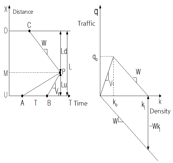
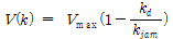
As shown in Diagram 1, Daganzo(1997) proposed Newell's 3-detector Simplification and a theoretical proof thereof. In this study, the description process of the model was revised through a review.

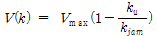
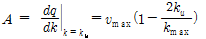
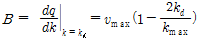
The NTSM assumes that in the continuum of three consecutive vehicle detectors(upstream, central and downstream detectors), there is no restriction on traffic volumes subject to upstream detection, whereas there are restrictions on traffic volumes subject to downstream detection, causing delays. Then, the traffic volume-density curve would be based on the simple triangle theory suggested by Newell(1993). Under these assumptions, the procedure of estimating a cumulative number of vehicles passing by a certain point (P) with a central detector installed(= theoretical cumulative traffic flow) is as follows.

First, as shown in Figure 1, since the upstream conditions are not so complex, there will be a characteristic curve with a gradient up to the point from the upstream detector. At the point of B, the wave expansion time, will be the previous time length.

Here,

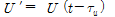
Under the characteristic formula conditions, the number of vehicles will not change and the number of vehicles on the central detector, calculated under the upstream conditions, will be the number of vehicles detected on the upstream detector prior to . Then, is independent from the conditions of traffic flows and, as in Figure 2, it will be , a result of the cumulative vehicle curve on the upstream detector. is moved to the right in parallel by . In this curve, if moved to the right, would be the virtual arrival curve on the point, .

Here,

On the other hand, for the downstream detector, a queue is formed, the wave shall is moved from point C to point P and the pulse velocity would be . Based on Figure 2 the slope, in line with the observer, is in parallel with the right side, Figure 2, where the q-k curve is in a queue. This means that the observed traffic volume is independent from the traffic conditions and it amounts to . Therefore, when a wave occurs on downstream and reaches the central detector, the change in number of vehicles observed is . This means that the change in number of vehicles observed equals to the number of vehicles between and at the critical density. It explains that the number of potentially observed vehicles based on the central detector under the downstream traffic conditions equals to the number of vehicles at the point . However, there will be a change about axis by hours ago and, on the axis, the cumulative traffic flow is increase by , the space of maximum interference. and are constants that are independent from the amounts of inflow and outflow. Hence, in conclusion, it will have the same effect as in case, when the curve is moved by to the top right by . The curve moved in parallel is in Figure 2. This s expressed as a potential departure curve in accordance with the downstream conditions. Then, the size of movement can be expressed as Vector . The vector elements are and . This means that the vector gradient is . Applying the Newell-Luke minimum principle, the number of vehicles actually observed pertains to the area below and . This area is shown in a thick line, in Figure 2. The crossed area of curves, and shows the route of shock waves on the detector. The shock waves occur as queues move forward and backward on the central detector, while the queue and non-queue statuses are repeated. 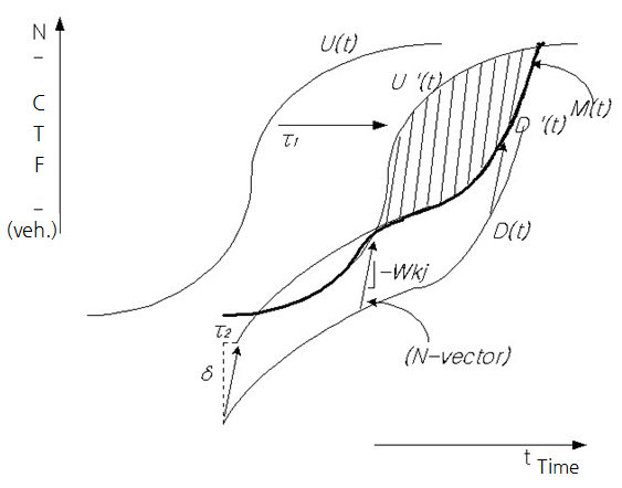Also, in Figure 2, the area between the curves and (deviant lines) indicates an area where vehicles experience a delay on M, upstream. Travel time can be divided into horizontal vectors, , , and and the cumulative number of vehicles consists of vertical vectors.

Methodology and Data Set-up

1. Fundamental Idea

The 3-detector simplification model used in this study was derived from an idea on the difference in density of traffics in an outbreak situation and a steady flow, which ultimately influence the relationship between traffic and density, having an impact on the traffic of the central detector of the 3-detector. Once an outbreak situation occurs, the shock wave will cause a fluctuation of density, resulting in a large error in measured accumulative traffic compared to the predicted. Such error of the estimated accumulative traffic, as detected by the central detector and the percentage error thereof will statistically significantly differ in a steady flow and in an outbreak situation. In this study, an idea of discriminating outbreak situations using the statistical significance was referred.

2. Building the Experimental Data

In order to collect the actual data, we used the Freeway Traffic Management System(FTMS) data within OASIS of the Korea Expressway Corporation. First, the data regarding accidents with trucks around Anseong, Gyeongbu Expressway(326km away from endpoint Busan) were collected to identify the conditions related to the accident, spots of accidents and time points. The data came from a time around 9 am, on Thursday 18th of September, 2003, based on the accident data. The analytic space covers 362.3-371.8km(approximately, 10km) from Busan, with reference to the highway distance in a time range from 8 am to 15 pm, including the moment of accident. The time range of steady traffic flows subject to a comparative analysis was between 8 AM and 15 PM, on Thursday, 25th of September, 2003, the same weekday and time range. The subject of analysis for data collection is as shown in Figure 3. The detector-based data pertaining to five spots from the rear of the accident spot were collected. The data that has errors in the raw data were omitted.

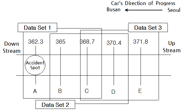
The highway VDS point-based data, including the spots of accidents on the road and time data, were applied as well. The data involve a loop detector of uploading traffic volumes, speeds and occupancy rates for every 30 seconds. The details of incidents occurred within the zone are as provided in Table 1.

3. The Procedure to Estimate Cumulative Traffic Flow on Central Detector

The procedure of estimating the theoretical Cumulative Traffic Flow() on a central detector, based on the CTFM, can be summed up as follows.

[STEP 0] Calculation of curves, cumulative traffic flows, upstream and downstream

[STEP 1] Calculation of traffic volumes starting from upstream()

  [STEP 1-1] Calculation of upstream density

  [STEP 1-2] Calculation of traffic volumes starting from upstream

[STEP 2] Calculation of traffic volumes arriving at downstream() = Traffic volume reduced from shock waves

  [STEP 2-1] Calculation of downstream density

  [STEP 2-2] Calculation of the traffic volume, downstream

[STEP 3] Calculation of pulse velocity()

  [STEP 3-1] Calculation of upstream shock wave

  [STEP 3-2] Calculation of downstream shock wave

  [STEP 3-3] Calculation of pulse velocity

[STEP 4] Calculation of , coordinates- converted values

  [STEP 4-1] Unit time detection at upstream

  [STEP 4-2] Unit time detection at downstream

  [STEP 4-3] Calculation of the queue length arising from interruption

[STEP 5] Calculation of with coordinates converted

  [STEP 5-1] Calculation of (virtual start curve)

  [STEP 5-2] graph floating

  [STEP 5-3] Calculation

  [STEP 5-4] graph floating

[STEP 6] Calculation of the theoretical curve, Cumulative Traffic Flow

4. Statistical Fitness Test Method using Errors of Estimated Cumulative Traffic Flows

The hypothesis of the verification of homogeneity between the two independent traffic flows(steady and incident flows) is as follows, with the estimated cumulative traffic flow as an input.

The procedure of verifying the significance of steady and incident traffic flows is as follows.

[STEP7] Calculation of errors between theoretical cumulative traffic flow () and actual cumulative traffic flow() on the central detector under steady flows and incidents.

  Errors in cumulative traffic flow, central detector, under steady flows:

  Errors in cumulative traffic flow, central detector, upon an incident:

 [STEP 7-1] Calculation of mean and standard deviation of under steady flows

 [STEP 7-2] Calculation of mean and standard deviation of upon an incident

[STEP 8] Verification of the significance between standard deviations of and within the significance level

[STEP 9] Decision of the incident conditions

 If there is a significance between and within the given confidence interval, it would be decided as a steady traffic flow(　selected). Or no significance, it would be decided as an incident traffic flow( selected).

Results from Incidents Analysis

1. Estimated Results from Central Detector based Cumulative Traffic Flows

The statistical values for the verification of suitability of the estimated and actually measured cumulative traffic values of the center were applied, based on the NTSM, Mean Percentage Square Error(MPSE), Root Mean Square Error(RMSE) and Theil's Inequality Coefficient. As a result, while the estimated values of the Cumulative Traffic Flow were inappropriate around D(milepost 371.8), values from the two remaining points were appropriate in general. Also, the estimated values were more accurate under steady flows, than in incident. The results are as shown in Table 2. The table for the NTSM provided by this study means that the statistical suitability rises as the segment is located in the middle.

Errors and error rates in the By-time Newell Cumulative Traffic Flow are as in Figure 4-Figure 6. At first as in Figure 4, After 8:54, when the accident occurred, a significant difference is observed between the errors in cumulative traffic flow of steady and incident traffic flows within the analysis zone and, at around 11, the error reached its maximum at 8%. After 11, the error of cumulative traffic flows and of incident traffic flows both gradually decreased, but there was an increase in the secondary errors after 12:30. This causes the secondary queues by failing to rapidly reacting to the unexpected incident.

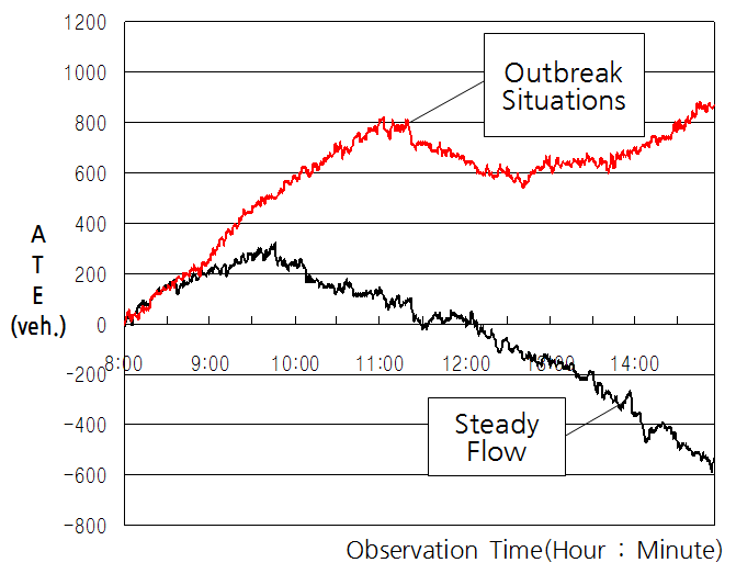
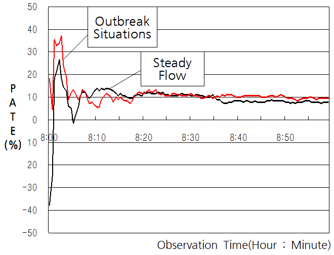
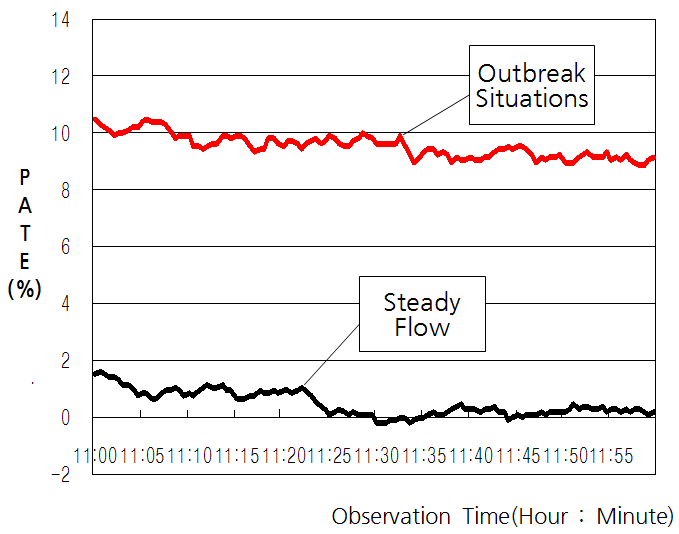
Figures 5 and 6 show the Percentage of Accumulated Traffic Errors(PATE) of the stage where errors for the accumulation traffic is shown at its maximum after an outbreak (Figure 6), and before the outbreak(Figure 5). Figure 4 differs for its axis of ordinates is composed of vehicles, while Figure 5 and 6's axis or ordinates are composed of percent values. The index idea for this study is to measure the difference in normal flow and accident flow by a certain unit(1 hour for this study) after measuring the percent unit of the error rate for accumulation traffic.

1. Results of Analysis of the Incident-involved Traffic Flow

Verification was accomplished on middle spot B and C where the estimated values of cumulative traffic flow were appropriately derived. The basic statistics under the theoretical cumulative traffic flows that are measured through the central detector under steady and incident traffic flows are displayed in Table 3 and Table 4. There is a great difference between the means of errors in the estimated and actual cumulative traffic flows on the central detector, under steady and incident flows.

Stated that Epsilon_B is error of the estimated accumulative traffic, in a steady flow and of the central detector at point B, and error of the actual accumulative traffic, Standard errors were 7.36 and 8.09 under steady and incident flows on Epsilon_B. Similarly, they were 7.36 and 13.74, respectively, on Epsilon_C.

Based on the null hypothesis, Folded F, the statistical value for verifying the homogeneity in error variances of cumulative traffic flows on the central detector under normal and incident traffic flows is found to be 1.21 on Epsilon_ B and 2.91 on Epsilon_ C, while the p value is less than 0.025, a critical value for rejection. It can be interpreted as the variance between the two traffic flows present a statistically significant difference. Accordingly, variances of errors in cumulative traffic flows under different conditions, divided into a steady flow and an incident, differ and they are necessary for confirming the results showing that the heteroscedasticity assumed variances are not equal to verify the differences in means. In this case, is 54.49 and P is below 0.0001, indicating the statistical differences in the means of error. Based on this, it is possible to interpret that the cumulative traffic flows, under a steady flow and an incident-led traffic flow, are heterogeneous in terms of their means and variances. This implies the cumulative traffic flow has characteristics that differ from those of steady traffic flow due to an incident, in which an error between the cumulative traffic flows becomes large enough for it to decide that there is a traffic flow with the characteristics that are different from those of an incident or a steady flow within that zone.

Conclusion and Further Study

In this study, it is assumed that the CTFM, suggested by Newell, is applied on the Cumulative Traffic Flow, which reflects the characteristics of dynamic traffic flows in the actual traffic environment, based on the data provided by the Korea Expressway Corporation's FTMS. In order to verify the feasibility of the assumed cumulative traffic flow, the errors in the Cumulative Traffic Flow were statistically analyzed and, based on the verification of heteroscedasticity of errors in cumulative traffic flows that was revealed from the central detector application between the steady flow and the incident-involved traffic flow, the study suggests a method of detecting all traffic flows involving the incidents, which differ statistically from the steady flows. The results of this study can be summarized as follows.

First, in this study, the CTFM is applied instead of the others detection methods of incidents, which enables estimating 30-seconds of cumulative traffic flows, in each of the incident and steady traffic flow, reflecting the dynamic changes in the traffic volume caused by shock waves. Also, the estimated outcomes could be the traffic flows of higher actual data and the statistical feasibility. Such result helped the authors to prove the statistical suitability of the NTSM. Second, based on the estimation Cumulative Traffic Flow as a variable to determine an incident, it was able to generally explore the traffic flow as an incident variable under the unexpected incidents, based on the changes in statistical errors in cumulative traffic flows. Based on the analytic results, the maximum error (8%) occurred around 11 o'clock, 2-3 hours after the accident. Lastly, in order to verify statistical significances in the incidents and steady traffic flows, T-Test and F-Test were conducted with the two traffic flows as independent variables. As a result, the accident-led incident traffic flow is found to have the heterogeneous characteristics, surrounding the dispersion and means of the steady traffic flows.

In order to derive the possible successive studies, first, there is a necessity for the calculation and settling based on continued studies and on-site data, for establishing an appropriate critical value to detect an incident accurately. Second, the boundary of the incidents on some of the closed zones on the Gyeongbu Expressway has caused difficulties in extracting the optimum data and the basic assumptions in this study to assume the traffic volumes. Thus there is a necessary for a continuous verification of the models pertaining to various incidents in broader range of time and space conditions, as well as the environmental variables. Third, the proposed technique used to detect the incident in this study need to be analyzed in comparison with other incidents-related algorithms, necessitating the measurement of detection rate, error rate and detection time and assessing the excellence of models thereof. Lastly, of the differences between the cumulative traffic flow of upstream and downstream in the Newell's mobile Cumulative Traffic Flow, in which the cumulative traffic flow detected in the upstream is higher than that in the downstream, explain that there are vehicles experiencing a delay within the zone. It is necessary to supplement the quantitative programs for calculating the number of vehicles that experience the queue and delay.