

Introduction
Data Description
1. Sites and Data
2. Preliminary Analysis of headway distribution across traffic states
Measurement Methodology
Analysis Results
1. Distribution of driver types
2. Effect of initial state on changes in driver characteristics
3. Effect of congestion severity
Conclusion
Introduction
Vehicle headways, both temporal and spatial, provide essential information on the macroscopic and microscopic features of traffic flow. First, they represent the distribution of vehicles on the road, which is related to the macroscopic flow rate. Therefore, we can estimate detailed variations in flow rate using headway analysis. Moreover, specific car-following behavior can be described from vehicle headways when traffic is in a congested state (Li and Chen, 2017). One notable car-following model is Newell’s simplified model (Newell, 2002), which assumes that speed and spacing have a linear relationship, as shown in Figure 1(a). We also derive the speed-headway curve from the definition of headway (= spacing/speed), as shown in Figure 1(b). These relationships are observed in many empirical analyses and presented in other models, though detailed parameters may differ. In a congested (= car-following) state, headway (spacing) decreases (increases) with increasing speed. However, in a free-flow state, where vehicles travel at their desired speed (or free-flow speed, V), headway depends on the random arrival of vehicles, with little influence from other vehicles. The dashed lines in both figures show that vehicles can exhibit any headway (spacing) exceeding the minimum headway (equilibrium spacing) in the free-flow state.
Meanwhile, advanced studies on car-following behavior have shown that the driver characteristic—the slope of the speed-spacing line (= reaction time, ) in Figure 1(a) is a dynamic parameter (Laval and Leclercq, 2010; Chen et al., 2012; Chen et al., 2014). Notably, Chen et al. (2014) categorize three driver characteristics as aggressive, Newell (neutral), or timid, and four driver reaction patterns as concave, convex, non-decreasing, and constant. Their study, verified using real-world NGSIM data (NGSIM, 2006), suggests that certain car-following behaviors may lead to the capacity drop phenomenon. While these studies effectively describe variations in driver characteristics, they do not clearly explain how or why drivers change those characteristics. In particular, most empirical verification of characteristic changes has been conducted within already congested traffic states(e.g., Oh and Yeo, 2015), and few studies have examined how driver characteristics change when traffic evolves from a free-flow to a congested state.
Thus, to fill this gap, this study employs high-resolution vehicle trajectory data extracted from drone videos to examine how the experience of traffic congestion alters driver characteristics across different traffic states, including the periods before, during, and after congestion. By analyzing car-following responses near bottlenecks, drivers are classified according to the extent of their behavioral adaptation, with particular attention to differences arising from the initial traffic state. This behavioral perspective is important because congestion-induced changes in driver characteristics, particularly shifts toward more timid driving, can degrade traffic efficiency and destabilize flow conditions. Understanding the origin of these behavioral adaptations provides valuable insights into traffic operation and flow stability, and offers a microscopic basis for explaining macroscopic phenomena such as capacity drop.
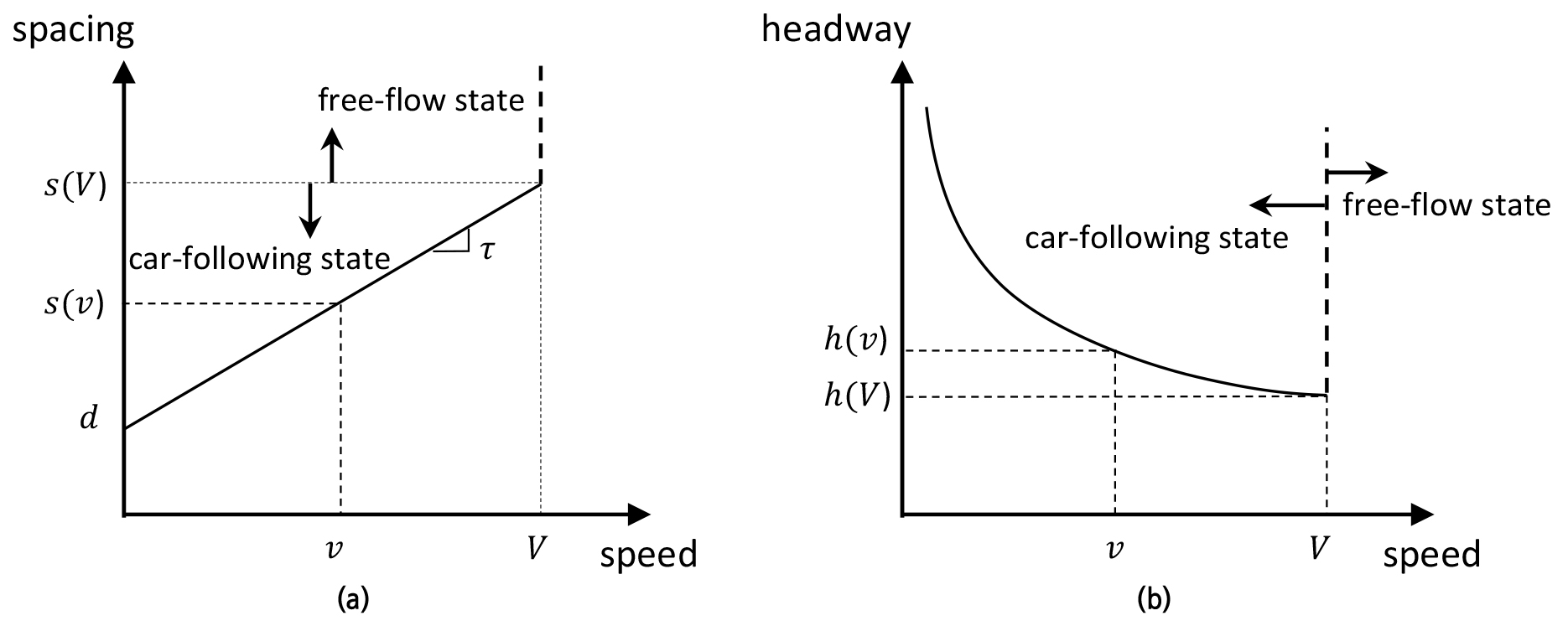
Figure 1
Newell’s Car-following model: (a) relationship between speed and spacing (adopted from Newell, 2002); (b) relationship between speed and headway
The rest of this manuscript is organized as follows. Section 2 describes the study sites and data. Section 3 and 4 presents the measurement methodology and the analysis results of changes in driver characteristics, respectively. Section 5 concludes the study and provides discussions.
Data Description
1. Sites and Data
The data consist of sets of vehicle trajectories extracted from drone videos, introduced in Han and Lee (2025). A swarm of three drones simultaneously recorded vehicle movement on two freeway sections in Seoul, as shown in Figure 2. The (red) dotted boxes in the figures indicate the bottleneck locations. The videos from each drone were merged into a single composite video. Figure 3 illustrates an example of the merged image from the three drones on the Gyeongbu (GB) Expressway. Using image analysis with deep learning algorithms, including YOLOv5, we identified the longitudinal and lateral coordinates of individual vehicles at 0.1-second intervals and constructed vehicle trajectories in the time–space domain for each lane. The extracted trajectories were repeatedly inspected and validated to ensure physical consistency, including checks for unrealistic vehicle overlaps, implausible overtaking events, and discontinuities in vehicle movement. Potential inconsistencies were corrected through iterative verification, ensuring that all trajectories used in the analysis satisfied basic physical and kinematic constraints. Table 1 summarizes the basic statistics of the collected data from both sites. Note that the drone recording periods were determined based on an analysis of 5-min aggregated traffic volume and speed data at each site. The results indicate that congestion at the GB Expressway typically emerges around 6:00 a.m. on weekdays, whereas at the Dongbu (DB) Expressway congestion develops gradually during the morning peak period rather than through an abrupt speed drop at a specific time. Considering these distinct congestion formation patterns, site-specific recording times were selected to capture representative traffic state transitions at each location. For further details on the data collection process and the observed traffic state transition observed at both sites, please refer to Han and Lee (2025). The data from the first site, the GB Expressway, capture the onset of traffic breakdown from a free-flow state at a freeway merge bottleneck, while the second site, the Dongbu (DB) Expressway, represents the aggravation of traffic congestion involving two separate bottlenecks. Since this study mainly aims to observe changes in driver characteristic as traffic evolves from a free flow state to congestion, the GB Expressway is used as the primary study area. The DB Expressway data serves as a comparison case to illustrate driver behavior under sustained congested conditions.
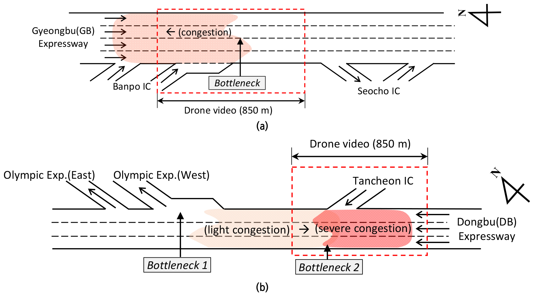
Figure 2
Sketch of the road sections (non-scale): (a) Site 1: Gyeongbu Expressway; (b) Site 2: Dongbu Expressway (adopted from (Han and Lee, 2025))
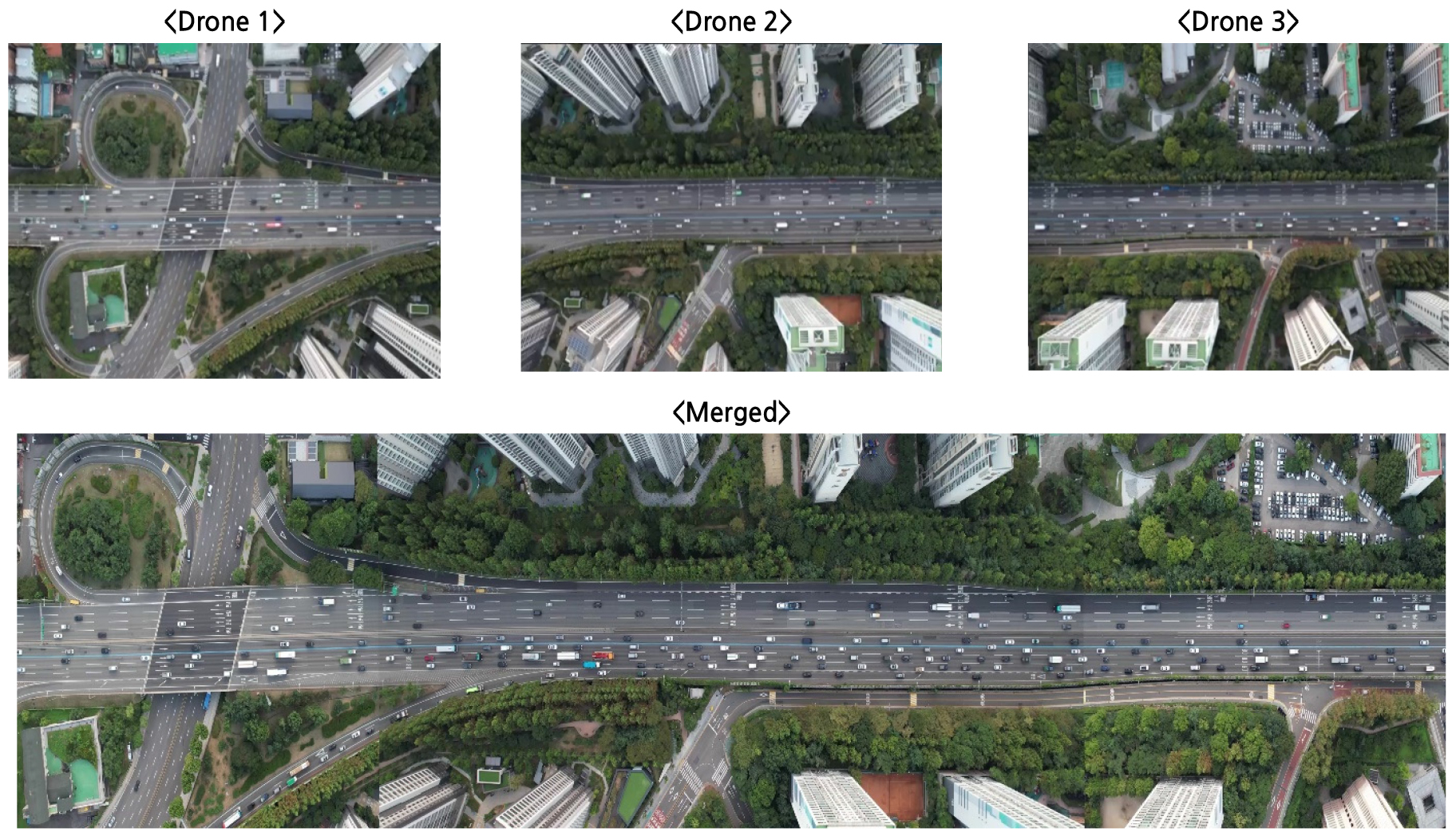
Table 1.
Basic statistics of the vehicle data
2. Preliminary Analysis of headway distribution across traffic states
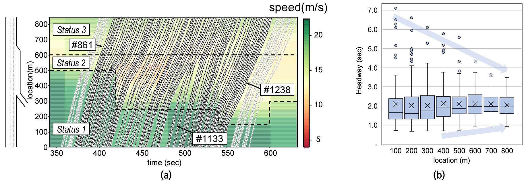
In this section, we conduct a preliminary analysis of how vehicle headways change in response to traffic state transitions. This analysis provides insights into the more detailed investigations presented in the following chapters. For this purpose, we use the trajectory data of vehicles between #861 and #1238 on lane one in Site 1. These vehicles represent a segment of traffic flow that experiences a transition from free-flow to congestion and then partial recovery. Figure 4(a) shows the trajectories of these vehicles, and Figure 4(b) presents the headway distributions as box plots by location. Specifically, the traffic flow can be divided into three distinct statuses as follows: (i) a free-flow state upstream of the bottleneck (Status 1), (ii) a congested state near the bottleneck (Status 2), and (iii) a recovered state downstream of the bottleneck (Status 3). The spatial ranges of Status 1 and Status 2 are dynamic due to the propagation of congestion, while the range of Status 3 is static (over 600m) and determined by the fixed bottleneck location.
In Status 1, the headway distributions reflect the features of random vehicle arrivals. The vehicle speeds – represented by the slopes of the trajectories in Figure 4(a) - are relatively uniform, while the headway distribution exhibits a wide range, as seen in the two box plots on the left in Figure 4(b). Meanwhile, in Status 2, vehicles begin to respond to their leading vehicles as they encounter a traffic disturbance. The headway range narrows significantly (see the four boxes at locations 300-600m in Figure 4(b)). In this status, vehicles decelerate to avoid collisions when their leaders slow down and accelerate when spacing increases. Further, in Status 3, downstream of the bottleneck, vehicle speed recovers - although not fully in this data set due to the limitations in the observation area. However, the range of headway distribution does not return to the level observed before congestion.
Specifically, two notable changes in the headway distribution are observed after congestion, as illustrated in Figure 4(b). First, large headways disappear, which is expected since they typically act as buffers that absorb traffic disturbance during congestion. Second, interestingly, the lower end of the headway distribution also shrinks. Before the breakdown point at 400m, headways under 1.5 seconds accounted for 23.9-40.0% of the observations, but this decreases to 9.9-14.0% between 600-800m.
Note that, according to general car-following (CF) models, headway is primarily a function of vehicle speed; therefore, headways are expected to return to their original distribution once speed is recovered after passing the. However, the persistent narrowing of the headway range suggests that drivers’ characteristics may have changed after experiencing traffic disturbance. In the following sections, we investigate whether this behavioral change is a general phenomenon in traffic flow under congested conditions.
Measurement Methodology
This section develops a measurement method to identify changes in driver characteristic using vehicle trajectory data. To this end, first, we assume (i) the vehicle’s behavior follows Newell's CF model, in which the following vehicle mimics the behavior of its leading vehicle. However, in the real world, a vehicle may behave differently from the expected trajectory, which is estimated based on a certain driver characteristic (specifically, the reaction time, τ, in Newell’s model) at a certain time. Therefore, building upon previous studies on dynamic driver characteristic, we further assume that (ii) the deviation between the actual and expected trajectory represents changes in driver characteristics.
Meanwhile, a key challenge in analyzing vehicle trajectories using the CF model lies in determining the precise moment when a vehicle transitions from a free-flow to a congested (car-following) state. As illustrated in Figure 1, most CF models simply assume that a car-following state begins when the vehicle’s speed is under the free-flow speed. However, this approach could lead to an overestimation of changes in driver characteristics. For example, vehicle #1133 in Figure 4(a) can be seen to reduce its speed below 80km/h (the speed limit) at time 503 seconds, in response to a decrease in the speed of its leading vehicle. According to general CF theory, vehicle #1133 may be considered in a car-following state after time 503 seconds. However, although its speed continues to decrease, the headway between vehicle #1133 and its leading vehicle also decreases, which is a feature of the free-flow state, or possibly an extreme change in driver characteristic. Thus, even though the speed is lower than the free-flow speed, the vehicle’s traffic state remains uncertain, suggesting the need for a more refined criterion for identifying the state transition point. When we recall the flow evolution in Section 2-2(Preliminary Analysis of headway distribution across traffic states), vehicles that pass the bottleneck area have three different statuses of free-flowing (at the bottleneck upstream), congestion suffering (within the bottleneck), and recovering (at the bottleneck downstream). The second and third statuses clearly represent car-following states, while the first remains uncertain. Accordingly, we propose the following assumptions: (iii) a vehicle is regarded to be in a car-following state only after its speed in Status 1 has decreased to a level comparable to the highest speed observed in Status 3. Note that the third assumption also enables a valid comparison of headways before and after congestion at similar vehicle speed.
Figure 5 illustrates the state definitions based on the above assumptions and the process of the proposed measurement method. First, we derive the driver characteristic before congestion, or reaction time, , from the vehicle’s speed () and actual headway () at the onset of the car-following state,, as:
where represents the wave speed. When the driver maintains his/her characteristic, the vehicle will follow the same trajectory as its leading vehicle, with a certain temporal and spatial difference, based on the first assumption. Accordingly, we can estimate the expected headways at the time of lowest speed, , and at the time of highest speed after experiencing congestion, , as:
where and represent the expected headway at and respectively. Note that these two time points, and , are selected to represent the change in driver characteristics during and after the experience of congestion, respectively. Then, the degree of change in driver characteristics can be quantified by comparing the expected and actual headway values at and as:
where and represent the ratio between the actual and expected headway values at and , respectively, and represents the difference between the actual and expected headway values at .
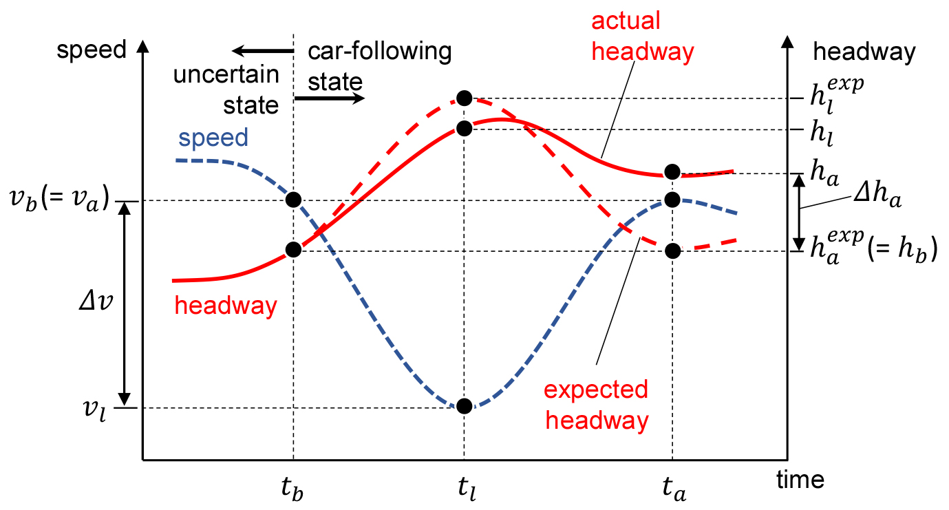
Figure 6 illustrates the four possible cases of changes in driver characteristics. First, when the driver maintains the same characteristic even after suffering a traffic disturbance, the actual headway will be similar to the expected headway. This case is denoted as Type Ⅰ. Meanwhile, when the actual headway is significantly larger than the expected one, it indicates that the driver has shifted toward a more timid characteristic (Type Ⅱ). Note that when drivers require additional headway, as in Type Ⅱ, the discharge rate from a congested area will decrease, leading to a capacity drop. By contrast, when the driver’s characteristic becomes more aggressive, the actual headway will be smaller than the expected headway (Type Ⅲ), which could increase the discharge rate. Lastly, when the vehicle travels in a free-flow (or uncertain) state during the entire study period, we categorize it as Type Ⅳ, as shown in Figure 6(b). Note that Type IV vehicles should be excluded from the following analysis, as they could skew the results related to change in driver characteristics; their headways decrease significantly after traffic disturbance, which could be regarded as an extreme case of Type Ⅲ, aggressive drivers.
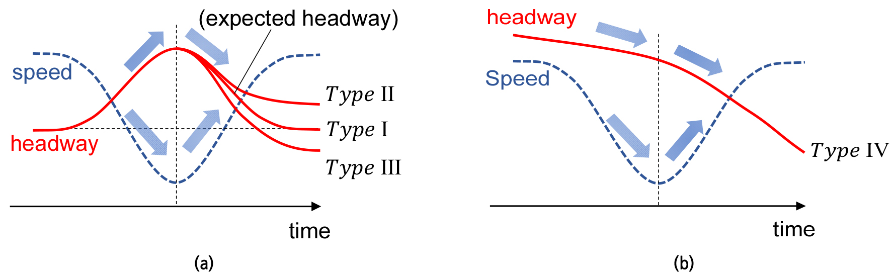
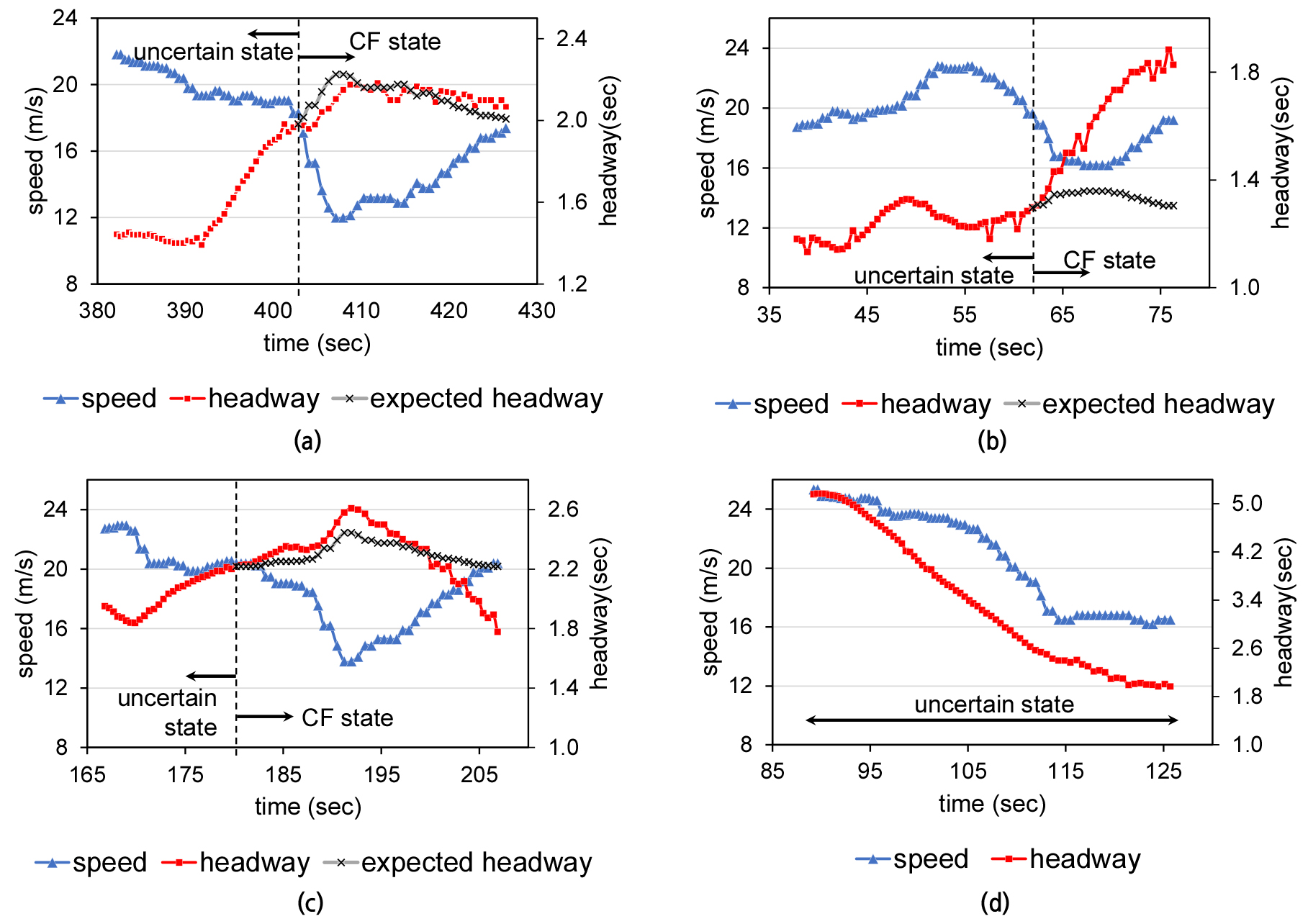
Figure 7 shows example cases for each type and their corresponding speed-headway relationship from the GB expressway. The following criteria, adopted with reference to previous studies on driver behavioral adaptation and car-following behavior (Chen et al., 2012, Chen et al., 2014), are used for classification: 0.9 1.1 for Type Ⅰ, 1.1 for Type Ⅱ, and 0.9 for Type Ⅲ. Type Ⅳ is categorized when the headway decreases continuously regardless of changes in speed.
Analysis Results
1. Distribution of driver types
We analyze the change in driver characteristics using the proposed method. The analysis is applied to data from both Sites 1 and 2 to identify how traffic flow features differ based on the initial traffic state. Figure 8 presents the distribution of driver types for both sites, showing that the characteristic distributions vary depending on the traffic state at the beginning. In Site 1, the proportion of Type Ⅱ drivers who increase their headway after suffering congestion is 44.2%, while the proportion of Type Ⅲ drivers who decrease the headway is only 18.5%. Thus, the overall average headway is expected to increase downstream of the bottleneck at Site 1. In contrast, at Site 2, the proportion of Type Ⅱ and Type Ⅲ drivers are both 38.5%, and the proportion of Type Ⅰ drivers who do not change their characteristics is 23.0%. Therefore, the effects of increased and decreased headway from Type Ⅱ and Ⅲ drivers are likely to offset each other, and the overall headway is expected to remain similar at Site 2. Note that Type Ⅳ drivers, who remain in a free-flow (or uncertain) state throughout the observation period, exist only at Site 1, comprising 6.6% of the sample.
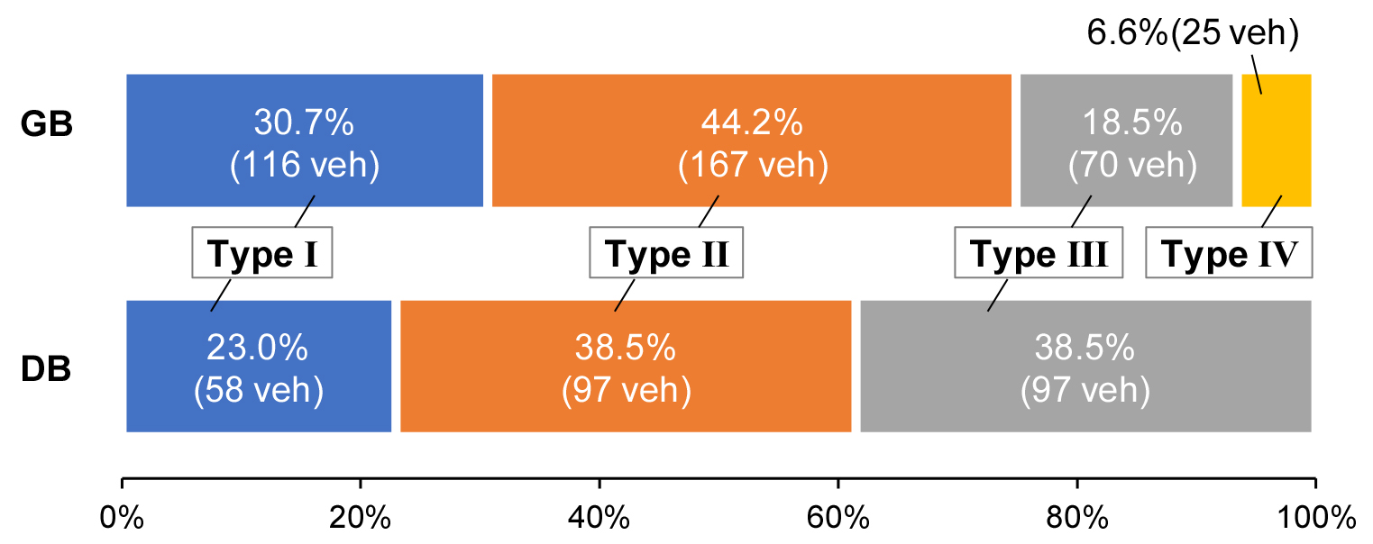
Table 2 presents the relationship between driver types and their aggregate effects on macroscopic traffic flow feature. In Site 1, the sum of for Type Ⅰ drivers is nearly zero, at -0.71 seconds across 116 vehicles, indicating that their overall impact on traffic flow is marginal. On the other hand, Type Ⅱ drivers increases their headways by 0.63 seconds per vehicle, resulting in a total increase of 105.32 seconds across 167 vehicles. Meanwhile, Type Ⅲ drivers reduce their headways by an average of -0.56 seconds, with a total decrease of -38.91 seconds for 70 vehicles. Consequently, the total headway increase for all 353 vehicles in Site 1 is 65.69 seconds over an observation period of 901.10 seconds. This implies that an additional 7.3% (=65.69/901.10) of time in the time-space domain is required downstream of the bottleneck to accommodate the same number of vehicles after suffering congestion. This result may reflect a reduction in the discharge rate, commonly known as the capacity drop phenomenon. On the other hand, the total in Site 2 is 19.27 seconds for 252 vehicles, corresponding to only 2.5% of the total analysis time of 780.0 seconds. This suggests that additional headway is less necessary in terms of car-following behavior when traffic is already in a congested state.
Table 2.
Headway change () by driver type
| Road | Type | Vehicles | (sec) | ||||
| Mean | Std. Dev. | Min | Max | Sum | |||
|
GB* (Site 1) | Ⅰ | 116 | -0.01 | 0.13 | -0.35 | 0.35 | -0.71 |
| Ⅱ | 167 | 0.63 | 0.55 | 0.13 | 4.16 | 105.32 | |
| Ⅲ | 70 | -0.56 | 0.42 | -2.04 | -0.11 | -38.91 | |
| Sum | 353 | 0.19 | 0.63 | -2.04 | 4.16 | 65.69 | |
|
DB (Site 2) | Ⅰ | 58 | -0.03 | 0.12 | -0.29 | 0.21 | -1.61 |
| Ⅱ | 97 | 1.00 | 1.02 | 0.16 | 3.66 | 96.9 | |
| Ⅲ | 97 | -0.78 | 0.49 | -2.21 | -0.20 | -76.02 | |
| Sum | 252 | 0.08 | 1.07 | -2.21 | 3.66 | 19.27 | |
2. Effect of initial state on changes in driver characteristics
This section investigates the effect of the initial traffic state – specifically, whether the traffic flow evolves from a free-flow state or not, on changes in driver characteristics by comparing the cases of different flow evolution. This study considers four distinct cases of traffic evolution. In Site 1(GB Expressway), vehicles initially travel in a free-flow state before evolving into congested state ( → ) and subsequently recovering from the congestion ( → ). These cases are referred to as GB1 and GB2, respectively. In contrast, vehicles in Site 2 (DB Expressway) also experience speed reduction due to evolving congestion, but all transitions occur within an already congested traffic state. These cases are referred to as DB1 ( → ) and DB2 ( → ). To examine the impact of speed change within the same site, we compare: ‘Pair 1: GB1 vs GB2’ and ‘Pair 2: DB1 vs DB2’. In addition, to assess the effects of the initial traffic state, we compare: ‘Pair 3: GB1 vs DB1’ and ‘Pair 4: GB2 vs DB2’. In each case, we compare the ratios or to evaluate how the driver characteristic changes in response to different traffic evolution scenarios.
Table 3 lists the statistical analysis results, and Figure 9 illustrates the distribution of (for GB1 and DB1) and (for GB2 and DB2) for each comparison pair. First, in Site 1, the changes in driver characteristics differ depending on whether vehicle speed is decreasing (GB1) or recovering (GB2). Specifically, the average value of for GB1 is 0.99 while the average of for GB2 is 1.16 (see Figure 9(a) for the distributions of and in Pair 1). The distribution and t-test result for Pair 1 show that the mean of for GB2 is significantly larger than the mean of for GB1. A Similar pattern is observed in Pair 2, which compares DB1 and DB2. These results indicate that vehicles tend to increase their headway after experiencing traffic disturbance, while they do not change significantly when the traffic state merely transitions into congestion.
Table 3.
T-test statistics for comparing groups
| Pair | Cases | Mean | Var. | n | df | t-value | t-critical (95%) | P value | ||
| 1-tail | 2-tail | 1-tail | 2-tail | |||||||
| 1* | GB1 | 0.99 | 0.05 | 353 | 352 | -11.041 | 1.649 | 1.967 | 0.000 | 0.000 |
| GB2 | 1.16 | 0.13 | 353 | |||||||
| 2* | DB1 | 0.97 | 0.16 | 252 | 251 | -6.266 | 1.651 | 1.969 | 0.000 | 0.000 |
| DB2 | 1.08 | 0.20 | 252 | |||||||
| 3** | GB1 | 0.99 | 0.05 | 353 | 371 | 0.534 | 1.649 | 1.966 | 0.297 | 0.594 |
| DB1 | 0.97 | 0.16 | 252 | |||||||
| 4** | GB2 | 1.16 | 0.13 | 353 | 471 | 2.075 | 1.648 | 1.965 | 0.019 | 0.038 |
| DB2 | 1.08 | 0.20 | 252 | |||||||
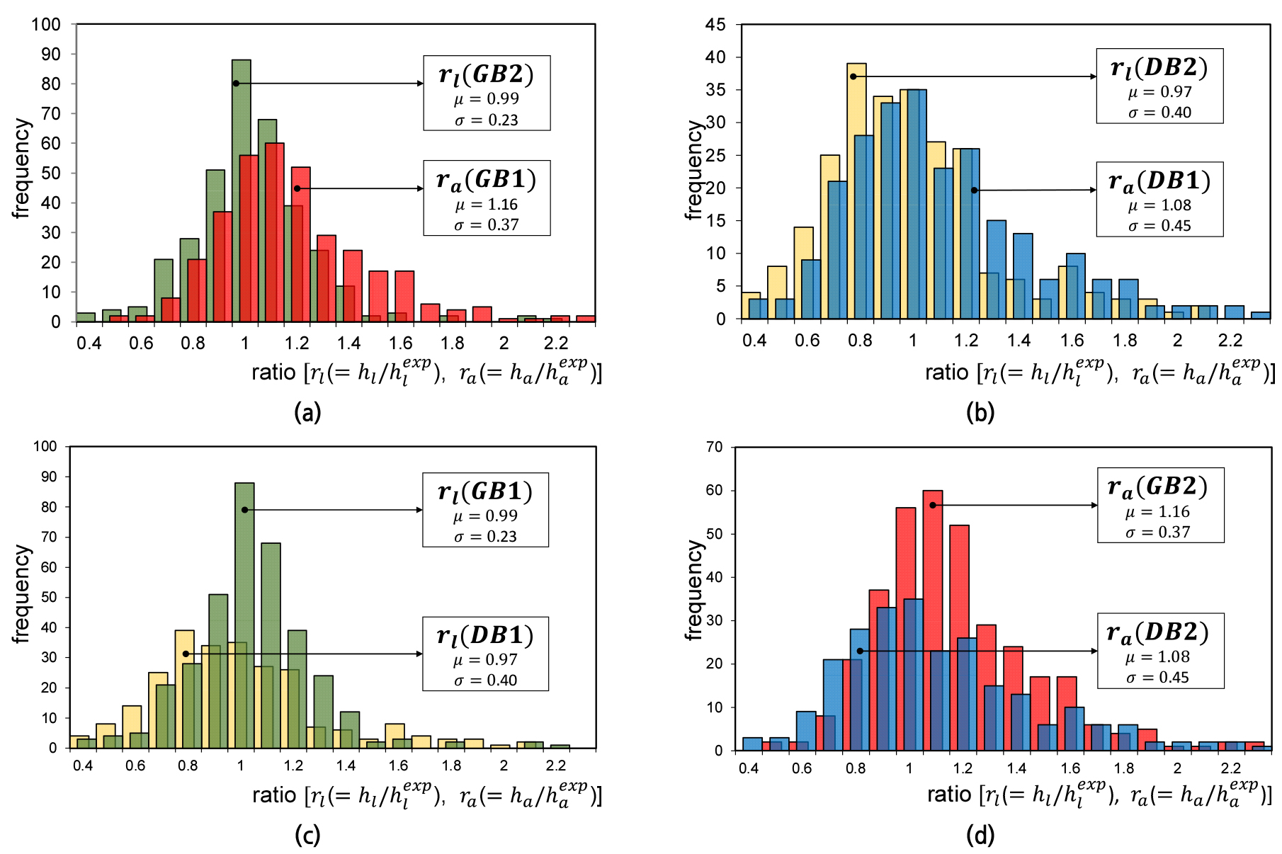
On the other hand, the degree of change in driver characteristics after congestion varies depending on the initial traffic state. This effect is highlighted in Pair 4 (GB2 vs DB2), as shown in Table 3 and Figure 9(d). In both cases, vehicles increase their headways after congestion, but the t-test result for Pair 4 shows that the mean of for GB2 is significantly larger than for DB2. This indicates that drivers become more timid, requiring larger headways, when the traffic flow initially originates from a free flow state, thus potentially leading to a larger reduction in discharge rate. In contrast, the analysis of Pair 3 (GB1 vs DB1) shows that the change in driver characteristics is similar regardless of the initial traffic state when the flow is transitioning into congestion. Therefore, through comparison of the four pairs, we find that drivers generally tend to increase their headway after experiencing congestion, and the degree of this change is significantly greater when the initial state is free flow.
Note that this finding differs from previous studies on the relaxation process, in which vehicles temporarily accepts short headways (or spacings) due to the maneuvering of lane-changing (LC) vehicles and gradually return to normal headways (or spacings) based on their speed (Zheng et al., 2013). Rather than focusing on short-term effects caused by LC maneuvers, our analysis examines longer term change across three traffic states: initial free flow, congestion, and recovery. Although some LC vehicles may trigger initial disturbance, most vehicles simply follow their leading vehicles according to their own (but dynamic) characteristics. Thus, car-following behavior and changes in drivers’ characteristics are the primary factors influencing headway differences before and after experiencing congestion.
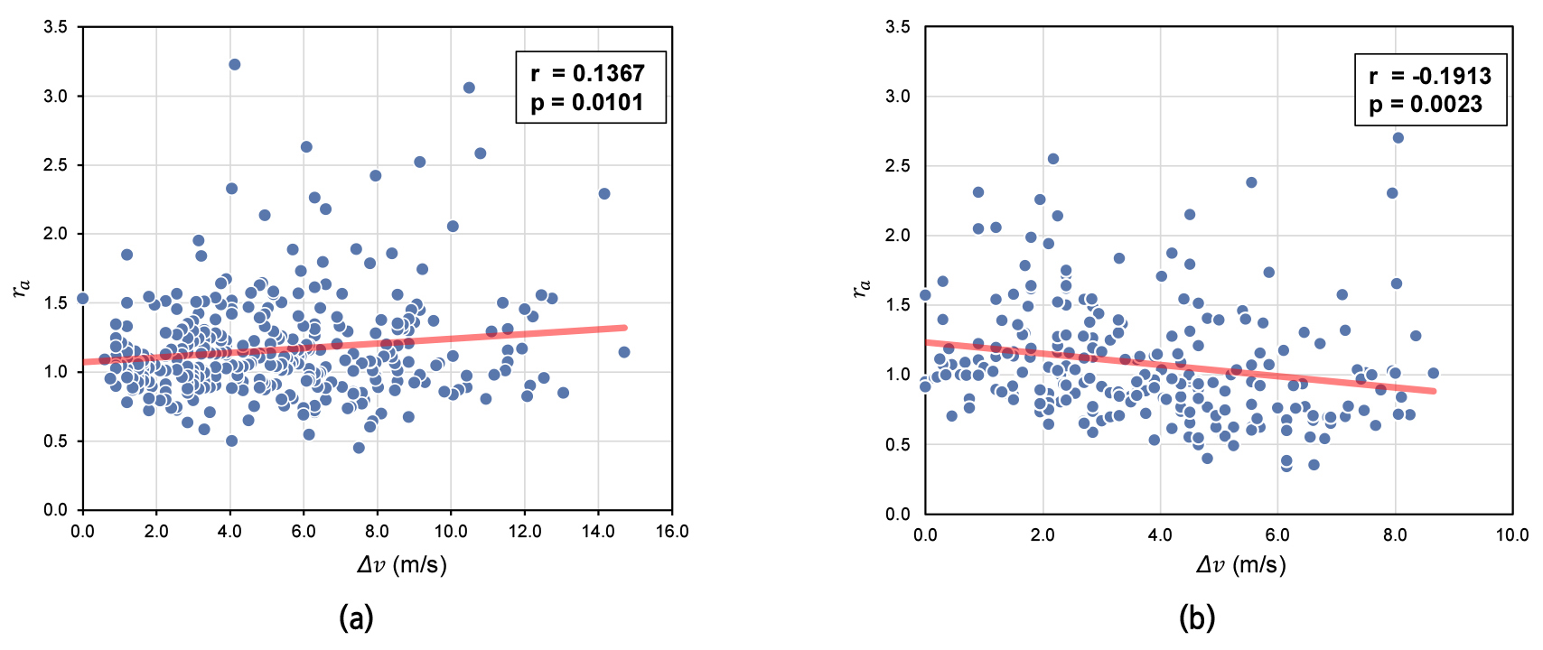
3. Effect of congestion severity
This section investigates the degree of change in driver characteristics with respect to congestion severity. Figure 10(a) presents the relationship between congestion severity, denoted as , and after experiencing congestion in Site 1. Note that a larger indicates a greater increase in headway, implying more timid driver behavior. The results show a weak but positive correlation between increase in headway and congestion severity (r = 0.137, p = 0.010). Although the magnitude of the correlation is small, a statistically significant directional relationship was observed. This suggests a consistent tendency for drivers to maintain larger headways as congestion severity increases, indicating more timid driving behavior. Interestingly, an opposite trend is observed when the traffic flow is already in a congested state. Figure 10(b) shows a weak but negative correlation between congestion severity and changes in driver characteristics (r = −0.191, p = 0.002). This indicates that, under sustained congestion, drivers tend to increase headway (i.e., become more timid) when the reduction in speed is small, whereas they are less likely to change their characteristic when the congestion severity increases. To better understand these contrasting trends, additional factors such as the duration of congestion and vehicle deceleration (or acceleration) patterns should be considered. Further data collection and analysis are required in future studies to clarify these behavioral response in detail.
Conclusion
This study revealed changes in driver characteristic as a result of experiencing traffic disturbance, particularly when traffic state transitions occur. To this end, empirical data were collected using drone videos that captured vehicle movement near freeway bottlenecks in Seoul. Based on Newell’s CF model, we estimated the expected headways during and after congestion, and compared them with the actual headways to identify changes in driver characteristics. We also analyzed the correlation between the degree of characteristic change and congestion severity. In particular, this study examined both traffics initially in a free-flow state and in a congested state to identify the distinct features associated with traffic state transition. The results show that drivers tend to secure larger headways, indicating more timid characteristics, after experiencing congestion, especially when transitioning from a free-flow state. The magnitude of this change also increases with the severity of congestion. From a macroscopic perspective, such behavioral changes imply that additional headways are required between vehicles after congestion, resulting in reduced discharge rates or capacity drops. However, those features were not observed when traffic evolved from an already congested state.
These findings offer valuable implications for developing traffic control strategies aimed at mitigating the impact of driver behavior in response to traffic disturbances. First, in case of unavoidable congestion due to excessive demand, gentle and gradual speed reductions are preferable, particularly in already congested conditions. This study suggests that speed reduction from a free-flow state can lead to inefficient traffic operations, and this effect will grow when speed differentials are greater. Conversely, when speed control is implemented within an already congested state, the impact on driver behavior is marginal. Thus, implementing speed control within congested conditions may be more effective from a CF behavior perspective. In this context, a sufficient level of speed difference is also necessary to maintain control effectiveness, as shown in the negative relationship between speed reduction and behavioral change in Figure 10(b). In addition, this study provides a novel advantage of existing traffic control measures, such as Variable Speed Limits (VSL). VSL strategies are typically designed to reduce flow rates into bottlenecks by lowering upstream speeds. The findings of this study suggest that, beyond this flow-regulating function, VSL can also help suppress the behavioral shift toward larger headways, thereby mitigating capacity loss.
Several issues merit further research. This study analyzed two bottleneck sites in Seoul; therefore, the generalizability of the findings may be limited. In particular, the observed behavioral patterns may depend on site-specific factors such as roadway geometry, local traffic regulations, driving culture, and the time-of-day characteristics under which the data were collected. Future studies using more comprehensive datasets from different cities, roadway types, and traffic conditions are needed to further examine the applicability and limitations of the proposed findings. In addition, although vehicle types were identified in the collected data, this study did not explicitly differentiate driver behavioral changes by vehicle type (e.g., passenger cars, trucks, and buses). Given that vehicle type is likely to play an important role in shaping driver characteristics and their adaptation to congestion, future studies should investigate heterogeneity in behavioral responses across different vehicle classes. Furthermore, while this study focused on CF behaviors, driver characteristics are also influenced by lane-changing (LC) behaviors. Future studies should consider the combined effects of CF and LC behaviors on traffic flow and driver adaptation. In addition, sensitivity analyses on the classification thresholds and model parameters are warranted to assess the robustness of the results with respect to alternative specifications.
